Practical 4 Visualising phylogenies in R
The aims of this practical are to introduce you to some of the fun ways you can visualise phylogenetic trees in R. The code and examples are based on Liam Revell’s book chapter here.
Note that some of these plots won’t work very well in RStudio. You may need to click the zoom button to see them, or resort to using the old R GUI instead.
REMEMBER
- Download all of the data for the practical into a folder somewhere on your computer.
- Set your working directory to this folder.
- Start a new script for this practical.
You will also need to install the following packages:
apephytools
First load the packages we need and the data.
library(ape)
library(phytools)
Later we will use some Greater Antillean Anolis lizard data to add data to a phylogeny. Before we can add data to our tree, we need to load the data.
anoledata <- read.csv("anole.data.csv", header = TRUE)

# Look at the data
str(anoledata)
## 'data.frame': 100 obs. of 23 variables:
## $ species : Factor w/ 100 levels "ahli","alayoni",..: 1 2 3 4 5 6 7 8 9 10 ...
## $ AVG.SVL : num 4.04 3.82 3.53 4.04 4.38 ...
## $ AVG.hl : num 2.88 2.7 2.38 2.9 3.36 ...
## $ AVG.hw : num 2.36 1.99 1.56 2.37 2.69 ...
## $ AVG.hh : num 2.13 1.75 1.39 2.05 2.32 ...
## $ AVG.ljl : num 2.85 2.71 2.32 2.9 3.38 ...
## $ AVG.outlever : num 2.75 2.62 2.26 2.83 3.29 ...
## $ AVG.jugal.to.symphysis: num 2.54 2.37 2.08 2.6 3.07 ...
## $ AVG.femur : num 2.74 2.07 2.17 2.48 2.8 ...
## $ AVG.tibia : num 2.69 2.02 2.09 2.34 2.69 ...
## $ AVG.met : num 2.25 1.54 1.55 1.87 2.18 ...
## $ AVG.ltoe.IV : num 2.55 1.88 1.73 2.26 2.53 ...
## $ AVG.toe.IV.lam.width : num 0.1795 0.0488 -0.5361 0.4904 0.8441 ...
## $ AVG.humerus : num 2.46 1.95 1.63 2.3 2.62 ...
## $ AVG.radius : num 2.27 1.69 1.4 2.09 2.34 ...
## $ AVG.lfing.IV : num 1.94 1.4 1.04 1.7 1.98 ...
## $ AVG.fing.IV.lam.width : num 0.0754 -0.0739 -0.755 0.3155 0.6584 ...
## $ AVG.pelv.ht : num 1.99 1.51 1.19 1.87 2.1 ...
## $ AVG.pelv.wd : num 1.71 1.419 0.946 1.752 2.014 ...
## $ Foot.Lam.num : num 3.28 3.43 3.2 3.58 3.72 ...
## $ Hand.Lam.num : num 2.87 3.08 2.73 3.16 3.24 ...
## $ Avg.lnSVL2 : num 3.94 3.74 3.48 3.93 4.36 ...
## $ Avg.ln.t1 : num 4.41 4 4.37 4.44 5.04 ...Now let’s visualise some phylogenies!
4.1 Loading your phylogeny and data into R
4.1.1 Reading in a phylogeny from a file
To load a tree you need either the function read.tree or read.nexus. read.tree can deal with a number of different types of data (including DNA) whereas read.nexus reads NEXUS files. elopomorph.tre is not in NEXUS format so we use read.tree.
fishtree <- read.tree("elopomorph.tre")4.1.2 Reading in a phylogeny that is already built into R
The bird and anole phylogenies are already built into R so we don’t need to read them in using read.tree. Instead we just use:
data(bird.orders)
data(anoletree)
4.2 Basic tree viewing in R
We’ll use the Elopomorpha (eels and similar fishes) tree to start as it is simple.
Let’s examine the tree by typing:
fishtree##
## Phylogenetic tree with 62 tips and 61 internal nodes.
##
## Tip labels:
## Moringua_edwardsi, Kaupichthys_nuchalis, Gorgasia_taiwanensis, Heteroconger_hassi, Venefica_proboscidea, Anguilla_rostrata, ...
##
## Rooted; includes branch lengths.str(fishtree)## List of 4
## $ edge : int [1:122, 1:2] 63 64 64 65 66 67 68 68 69 70 ...
## $ Nnode : int 61
## $ tip.label : chr [1:62] "Moringua_edwardsi" "Kaupichthys_nuchalis" "Gorgasia_taiwanensis" "Heteroconger_hassi" ...
## $ edge.length: num [1:122] 0.0105 0.0672 0.00537 0.00789 0.00157 ...
## - attr(*, "class")= chr "phylo"
## - attr(*, "order")= chr "cladewise"fishtree is a fully resolved tree with branch lengths. There are 62 species and 61 internal nodes. We can plot the tree by using the plot.phylo function of ape. Note that we can just use the function plot to do this as R knows if we ask it to plot a phylogeny to use plot.phylo instead!
plot(fishtree, cex = 0.5)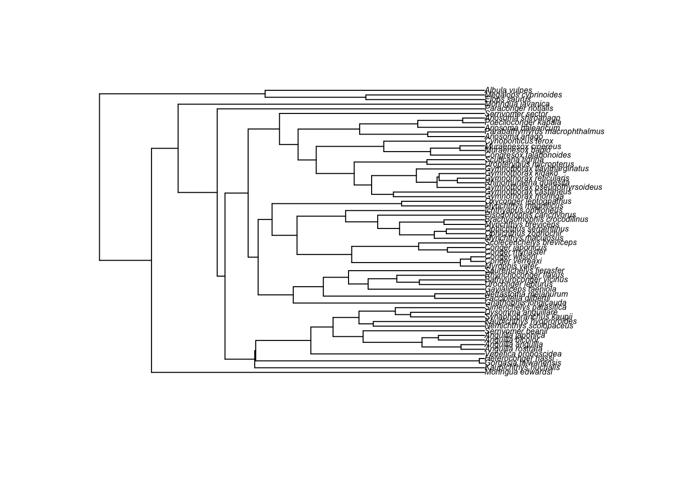
cex = 0.5 reduces the size of the tip labels so we can read them. We can also zoom into different sections of the tree that you’re interested in:
zoom(fishtree, grep("Gymnothorax", fishtree$tip.label), subtree = FALSE, cex = 0.8)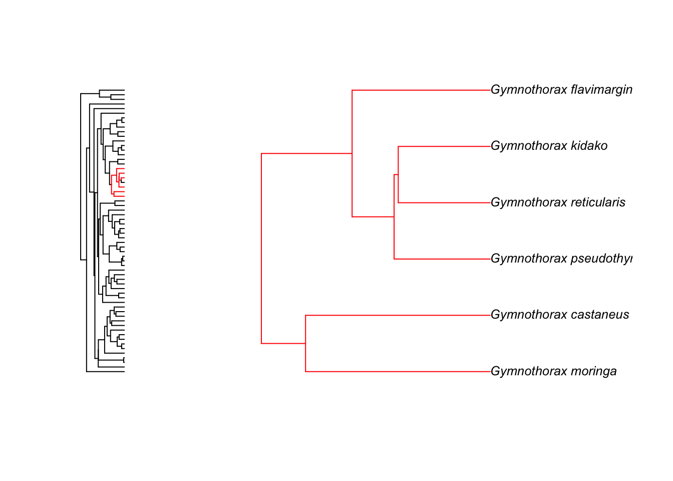
This just gives you the tree for Micropterus species but you can also see how the species fit into the rest of the tree using:
zoom(fishtree, grep("Gymnothorax", fishtree$tip.label), subtree = TRUE, cex = 0.8)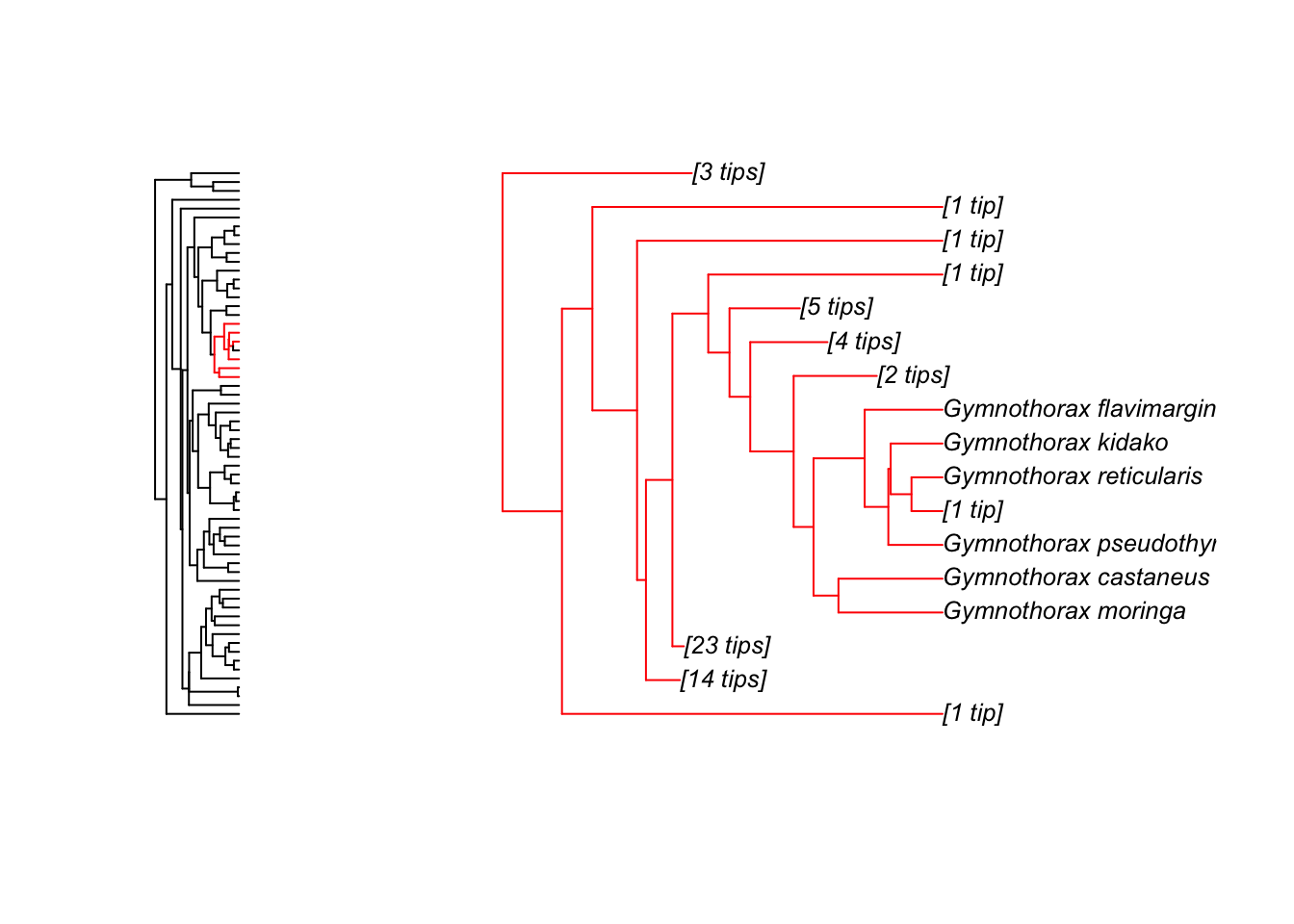
Note that zoom automatically sets the plotting window to display two plots at once. To reset this to one plot only use:
par(mfrow = c(1, 1))To get further options for the plotting of phylogenies:
?plot.phyloNote that although you can use plot to plot the phylogeny, you need to specify plot.phylo to find out the options for plotting trees. You can change the style of the tree (type), the color of the branches and tips (edge.color, tip.color), and the size of the tip labels (cex). Here’s an fun/hideous example!
plot(fishtree, type = "fan", edge.color = "deeppink", tip.color = "springgreen",
     cex = 0.5)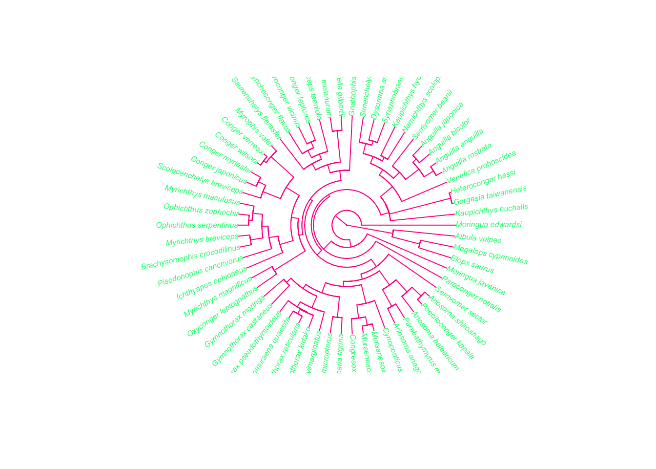
Or try
plot(fishtree, type = "c", edge.color = "darkviolet", tip.color = "hotpink",
     cex = 0.5)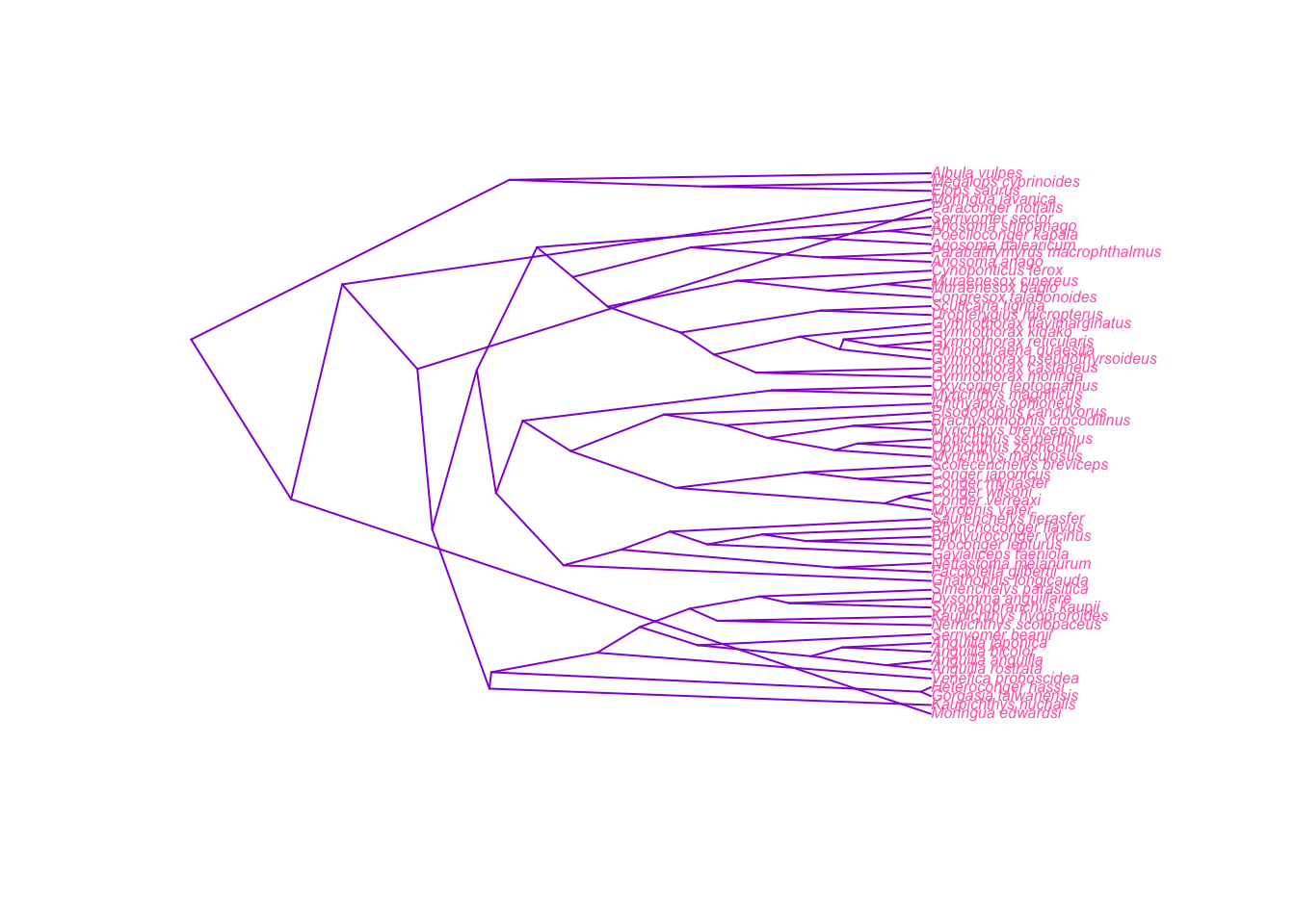
4.3 Adding trait data to trees in R
Note that the theory behind this is covered in more detail in the “Macroevolutionary Models in R” practicals part 1 and 2. ### Ancestral state reconstructions on discrete data We will use the bird data. Remember we already loaded the phylogeny and data as follows:
data(bird.orders)First we will invent some data for each bird order that we can reconstruct along the tree. This creates three variables, 0, 1 and 2.
mydata <- factor(c(rep(0, 5), rep(1, 13), rep(2, 5)))
mydata
## [1] 0 0 0 0 0 1 1 1 1 1 1 1 1 1 1 1 1 1 2 2 2 2 2
## Levels: 0 1 2We can then use the ape function ace to reconstruct ancestral characters along the nodes of the tree. type = d means the character to be reconstructed is discrete.
ancestors <- ace(mydata, bird.orders, type = "d")Now we can plot this on a phylogeny. First decide which colours we’d like. To look at a list of colours in R type in colors().
colours <- c("cornflowerblue", "cyan4", "goldenrod")Now plot the tree and add labels to the tips and the nodes using the results in ancestors. We use label.offset = 1 to move the labels to the right a bit so the pie charts will fit…
plot(bird.orders, label.offset = 1)
tiplabels(pch = 21, bg = colours[as.numeric(mydata)], cex = 2, adj = 1)
nodelabels(pie = ancestors$lik.anc, piecol = colours)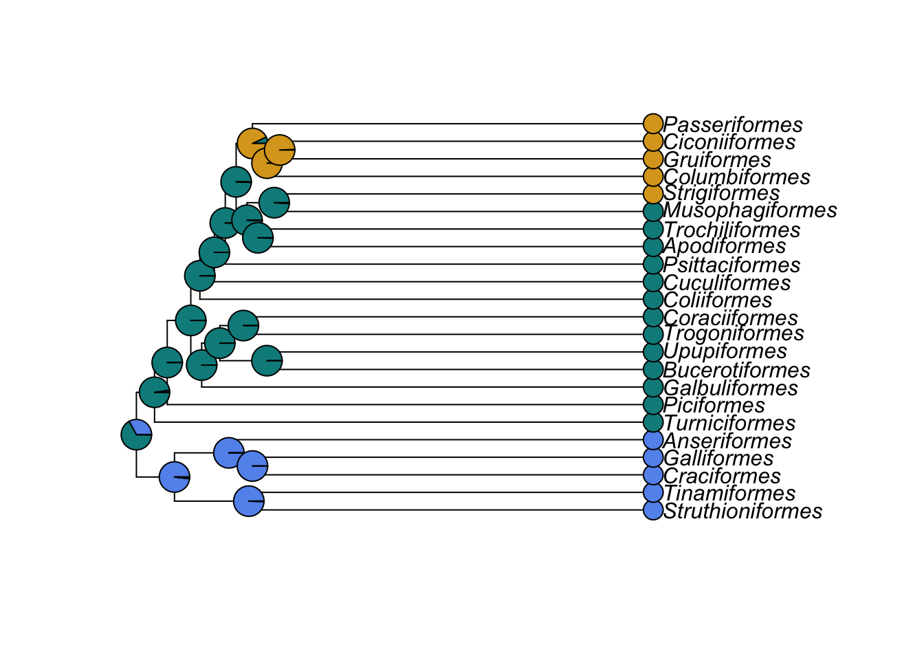
pch = 21 sets the tip labels to be unfilled circles, bg defines the colours of the circles using the list of colours we provided, and ordering them based on what the species value was for mydata (i.e. 0, 1 or 2). cex = 2 doubles the point size, and adj = 1 moves the tip labels sideways so they don’t obscure the ends of the branches. pie makes pie charts coloured using the ancestral state reconstructions in ancestors, and piecol tells it to use the colours we have defined.
4.3.1 Ancestral state reconstructions on continuous data
We are going to use the Anolis data to create a phylogeny with different colours for different observed and reconstructed body sizes (snout-to-vent length, SVL). Remember we already loaded the phylogeny and data as follows:
data(anoletree)
anoledata <- read.csv("anole.data.csv", header = TRUE, row.names = 1)
Note the names in anoledata are the species names without the Genus. In the phylogeny the species names are Anolis_species. So to get the two to match we need to add Anolis_ to each name.
rownames(anoledata) <- paste("Anolis", rownames(anoledata), sep = "_")paste just sticks together Anolis with the names in anoles already with an underscore (_) separating them (sep = "_")
We then need to make sure the order of the species in the data matches that of the phylogeny.
anoledata <- anoledata[anoletree$tip.label, ]Next we make a matrix containing only the SVL values for each Anolis species:
SVL <- as.matrix(anoledata)[,"AVG.SVL"]This code selects only the variable AVG.SVL from anoledata (square brackets subset in R in the form [rows, columns]), and then uses as.matrix to make this into a matrix.
Take a look at SVL
head(SVL)## Anolis_ahli Anolis_allogus Anolis_rubribarbus
## 4.039125 4.040138 4.078469
## Anolis_imias Anolis_sagrei Anolis_bremeri
## 4.099687 4.067162 4.113371We then use the function contMap. contMap creates a tree with a mapped continuous character, i.e. where the value of the character is known at the tips, and estimated along the tree. The estimating of the character along the tree uses a Maximum Likelihood estimation procedure. Here we will tell contMap not to automatically plot the tree (using plot = FALSE) so we can make some modifications.
SVLplot <- contMap(anoletree, SVL, plot = FALSE)Finally let’s plot the tree as a fan (legend = 10 just spreads the legend out so it is readable).
plot(SVLplot, type = "fan", legend = 10)## legend scale cannot be longer than total tree length; resetting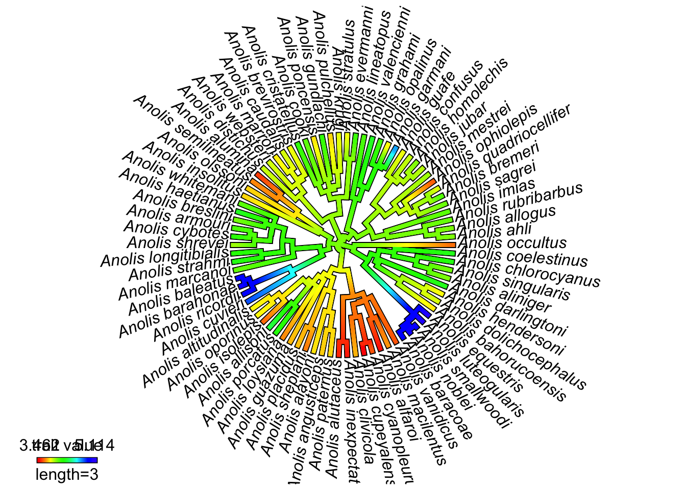
4.4 Phylomorphospace plots in R
We are going to use the Anolis data to create a phylomorphospace plot. These plots show where species fall within a morphospace (usually based on principal components analyses of morphological variables), and then reconstructs values for the nodes of the phylogeny so the whole phylogeny can be projected into the morphospace.
We already loaded the phylogeny and data as follows:
data(anoletree)
anoledata <- read.csv("anole.data.csv", header = TRUE, row.names = 1)
As we saw above, the names of anoles are the species names without the Genus. In the phylogeny the species names are Anolis_species. So to get the two to match we need to add Anolis_ to each name.
rownames(anoledata) <- paste("Anolis", rownames(anoledata), sep = "_")paste just sticks together Anolis with the names in anoles already with an underscore (_) separating them (sep = "_")
Next we again need to make sure the order of the species in the data matches that of the phylogeny.
anoledata <- anoledata[anoletree$tip.label, ]We can now run a phylogenetic principal components analysis on our morphological trait data and extract the PC scores for each PC axis using $S.
PC <- phyl.pca(anoletree, anoledata)$STo plot the morphospace with colours, we need to define them. Here we choose six colours, and matched them with the ecomorph types listed here. These were built into anoletree.
colors <- setNames(c("cornflowerblue", "goldenrod", "chartreuse", "hotpink",
                     "orangered", "darkviolet"),
                     sort(unique(getStates(anoletree, "tips"))))
Finally we can make the plot, and colour by ecomorph. label = "off" suppresses the printing of tip labels which keeps things a bit tidier.
phylomorphospace(anoletree, PC[,1:2], label = "off", node.by.map = TRUE, colors = colors)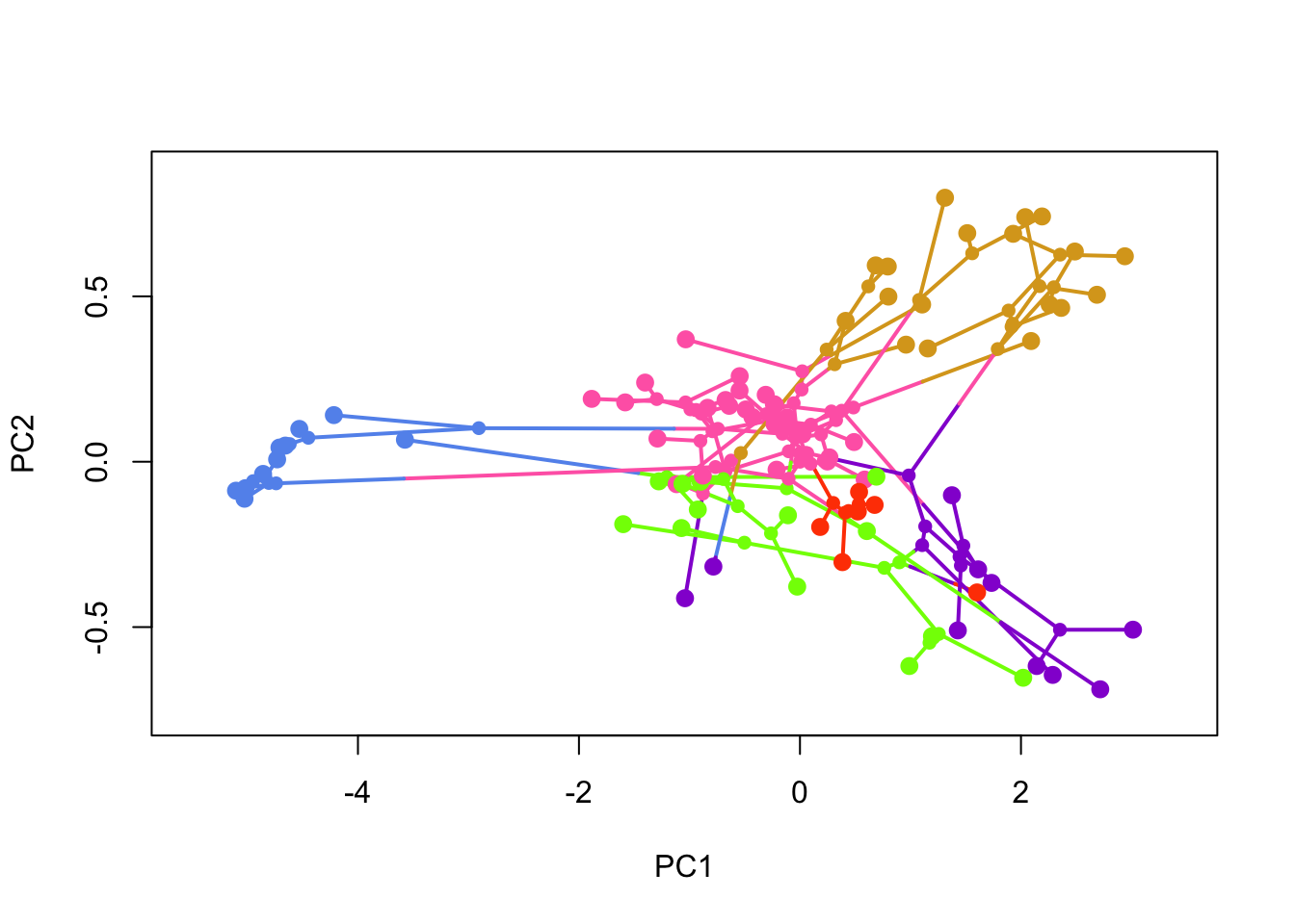
4.5 Phylogenies and maps!
We can also plot phylogenies attached to maps showing where species come from. We will use the bird orders tree again as it’s small.
data(bird.orders)We don’t know where the birds come from, so we will simulate some latitude and longitude data as follows. This uses a function that simulates traits along the phylogeny, so close relatives should end up with more similar latitude and longitude values. I’ve used high rates of evolution (sig2) to force the points to be spread out. Of course these values will be nonsensical for birds!
lat <- fastBM(bird.orders, sig2 = 100, bounds = c(-90, 90))
long <- fastBM(bird.orders, sig2 = 150, bounds = c(-180, 180))
Then we use the function phylo.to.map to match the locations with the world map. This produces some output in the form objective 98 etc. (I have suppressed it here).
phylomap <- phylo.to.map(bird.orders, cbind(lat,long), plot = FALSE)We can either put the phylogeny next to the map and draw lines to the places they come from using type = "phylogram"…
plot(phylomap,type = "phylogram", asp = 1.3, mar = c(0.1, 0.5, 3.1, 0.1))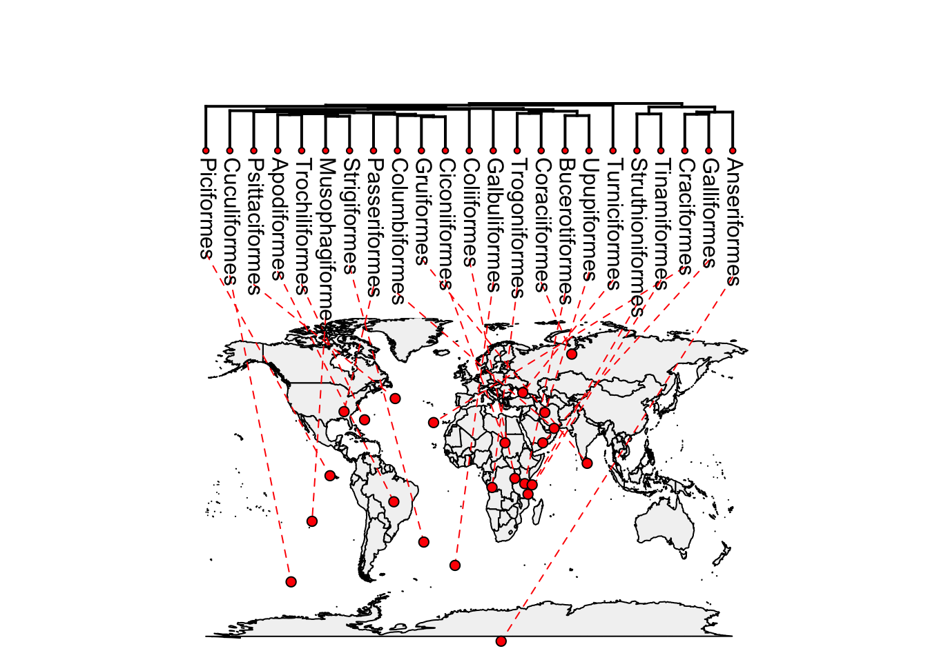
…or plot the phylogeny directly onto the map using type = "direct"
plot(phylomap,type = "direct", asp = 1.3, mar = c(0.1, 0.5, 3.1, 0.1))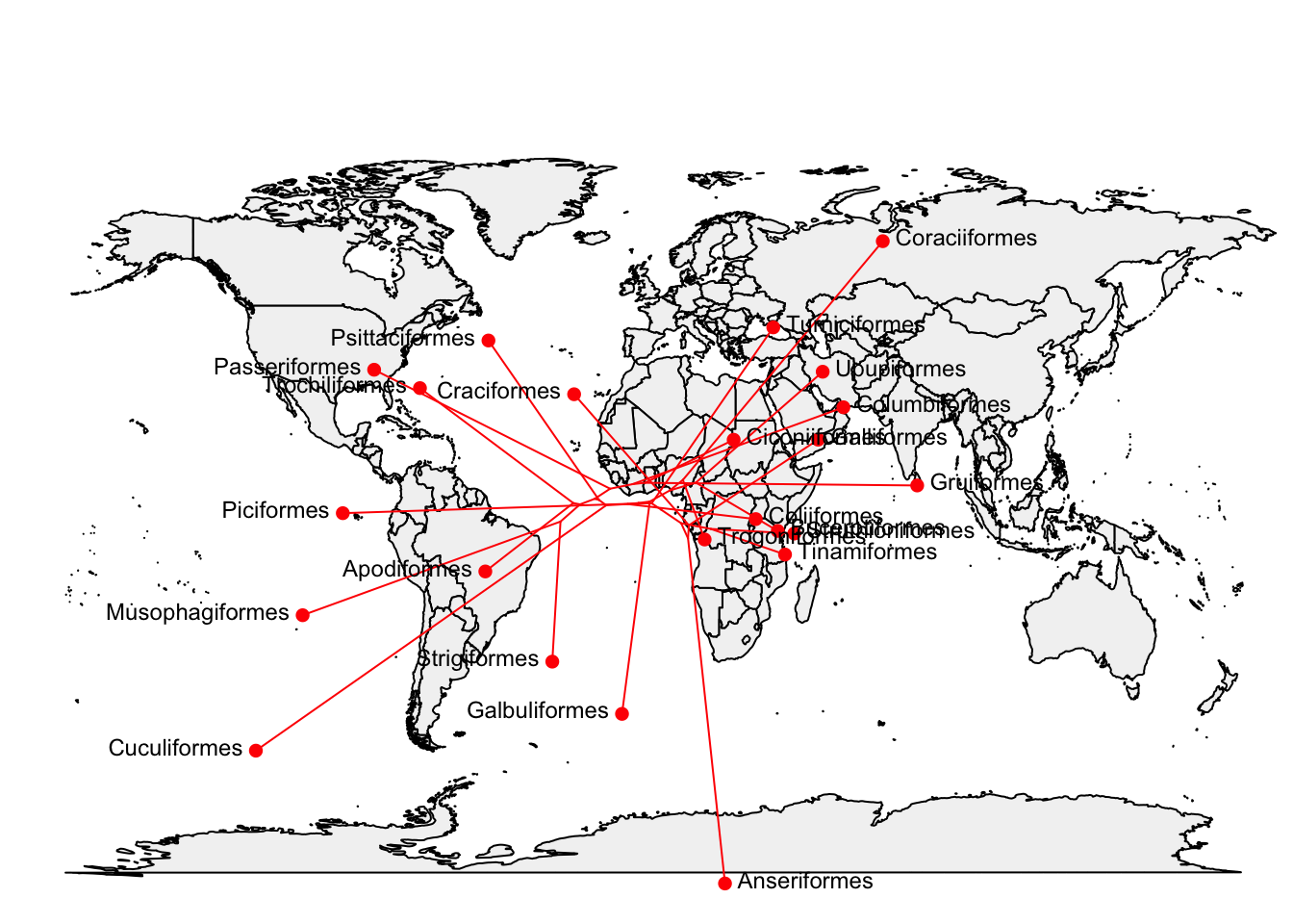
4.6 A new package for visualising trees: ggtree
ggtree is a newly released package that works with the popular ggplot framework in R. ggplot works by adding layers of different features together. A standard ggplot includes a layer that assigns the x and y variables then can have lots of other layers of points, lines, shapes and now with ggtree phylogenies.
Unfortunately this is broken in the most recent version of R. I’ve left this in, just in case they fix it soon
To use ggtree you will have to install it, then load it using:
library(ggtree)Let’s replicate some of the stuff we did above but using ggtree. As always choose whichever method you prefer when you’re doing this with your own data.
ggtree(fishtree) +
geom_text(aes(label=label), size = 1)
Note that the layers here are the tree, and then the tip labels. Layers are separated by +
We can also zoom in on sections like with ape.
gzoom(fishtree, grep("Gymnothorax", fishtree$tip.label))And we can have different shapes of phylogeny, different colours and even different line types.
ggtree(fishtree, color = "steelblue")
ggtree(fishtree, layout = "circular")
ggtree(fishtree, linetype = "dotted")
ggtree is really great for highlighting sections of a tree. First look at the nodes on your tree and pick an interesting one…
ggtree(fishtree) +
  geom_text(aes(label = node))
Then highlight and/or annotate…
ggtree(fishtree) +
geom_hilight(node = 73, fill = "steelblue", alpha = 0.6) +
geom_hilight(node = 97, fill = "darkgreen", alpha = 0.6)
This package has a huge amount of promise, but still a few bugs and weird features (it’s designed by geneticists who are used to dealing with short species labels, hence the issues getting our species names to actually fit on the plot). The help files are also currently a bit sparse and some of the vignette examples don’t work. But if you’re likely to need to do any of this kind of stuff I recommend checking out the vignette and the paper:
- Guangchuang Yu, David Smith, Huachen Zhu, Yi Guan, Tommy Tsan-Yuk Lam. ggtree: an R package for visualization and annotation of phylogenetic trees with their covariates and other associated data. Methods in Ecology and Evolution 2016, doi:10.1111/2041-210X.12628.