Practical 7 Macroevolutionary models in R: Part 2 - discrete traits

The aims of this practical are to learn how to use R to fit macroevolutionary models in R to discrete traits.

We will be using the evolution of magical creature life-history variables as an example. The data includes body mass (average adult size at rest) in kg, social status (1 = solitary, 2 = social), habitat (1 = terrestrial, 2 = aquatic, 3 = volant) and magical power (in thaum - with thanks to Terry Pratchett for the units). These data are invented, so please don’t get too upset if I’ve misclassified anything!

REMEMBER

Download all of the data for the practical into a folder somewhere on your computer.
Set your working directory to this folder.
Start a new script for this practical.

You will also need to install the following packages:

ape
geiger
OUwie

This is Part 2 of the “Macroevolutionary models in R” practical, so you can skip through the set up if you’re just carrying on from that.

This handout borrows heavily from a Linnaean Society workshop I ran with Graham Slater in 2014. Many thanks to Graham for his invaluable input.

7.1 Preparing for the analysis

7.1.1 Load packages, read in the data and the tree

This is the same as we did in the PGLS practical, so I won’t give detailed instructions here.

# Load packages
library(ape)
library(geiger)
library(OUwie)

# Read in data
magicaldata <- read.csv("magicalcreatures.csv")
# Check data is loaded correctly
str(magicaldata)

## 'data.frame':    30 obs. of  5 variables:
##  $ Species     : Factor w/ 30 levels "Acromantula",..: 22 24 19 5 7 16 21 25 30 29 ...
##  $ BodySize_kg : num  1.5 50 0.5 100 8000 1 2.5 6 800 600 ...
##  $ SocialStatus: int  2 2 2 1 1 2 2 1 1 2 ...
##  $ Habitat     : int  1 1 2 1 3 1 1 3 3 3 ...
##  $ Magic_thaum : num  106.3 86.7 98.6 57 131.9 ...

# Read in tree
magicaltree <- read.nexus("magicaltree.nex") 
# Check tree is loaded correctly
str(magicaltree)

## List of 4
##  $ edge       : int [1:52, 1:2] 28 29 30 31 31 30 32 33 33 34 ...
##  $ edge.length: num [1:52] 136.86 65.69 97 2.92 2.92 ...
##  $ Nnode      : int 26
##  $ tip.label  : chr [1:27] "Doxie" "Bowtruckle" "Hinkypuff" "Grindylow" ...
##  - attr(*, "class")= chr "phylo"
##  - attr(*, "order")= chr "cladewise"

7.1.2 Modify the tree and data so they can be used in the analyses.

Again we did this in the PGLS practical. Please remind yourself of what these steps are needed for.

# Ensure tree is fully bifurcating
magicaltree <- multi2di(magicaltree) 

# Replace spaces with underscores in the species names
magicaldata$Species <- gsub(" ", "_", magicaldata$Species)

# Add species names to row names
row.names(magicaldata) <- magicaldata$Species

For some weird reason the geiger function we need (treedata see below) won’t work if you input a dataset with variables that are characters i.e. words or letters. Our taxonomic variable Species is a character so we need to exclude it from the data. Note for your own data you’d need to remove all character variables (or recode them as 0,1,2 etc.). We will do this by making a new dataset called magicaldata2.

magicaldata2 <- magicaldata[, 2:5]

Here the [ ] tells R we want to subset the dataset. R data frames are always described by [X, Y] where X is rows and Y is columns. So [1, 1] will select the entry in the first column and the first row of the data frame. [, 2:5] selects all rows but only columns 2 to 5. These are the columns containing our numeric variables.

We then need to match the species in tree to those in the dataset as in the PGLS practical. Note that we are using magicaldata2 here.

match.species <- treedata(magicaltree, magicaldata2)

mytree <- match.species$phy
mydata <- match.species$data

7.2 Fitting models of evolution to discrete data (regime dependent evolution)

In the previous section we saw how to fit three models of trait evolution to continuous variables. Although the evolutionary modes seem quite different, all are similar in that the evolutionary process is constant over the entire clade, i.e., all branches are evolving at the same rate (in BM), drawn to the same trait value with the same strength (OU) or decline in rate at the same time-dependent pace (EB). Often, we want to relax this assumption. Members of our clade might belong to one of a set of ecological regimes, for example dietary niches or locomotor modes, and we might hypothesize that there are different evolutionary rates or different optimal trait values for each of these regimes. In this section, we’ll look at how to fit these kinds of models using the OUwie package.

First we will look at how to reconstruct the evolutionary history of a discrete trait. Then we will use OUwie to allow rates and optimal trait values for a continuously valued trait, like body size, to vary, based on that discrete trait.

Here we will use the discrete variable SocialStatus from our magical creature dataset. Any species with a social group size of 1 is solitary (SocialStatus = 1), while any species with a group size greater than 1 is social (SocialStatus = 2).

We can visualize these variables on our tree by plotting them with colors. We’ll use light blue for solitary and plum for social. Because our states are coded as “1” and “2”, we can use a little trick to get the appropriate colors by indexing a vector of “lightblue” and “plum”. We first need to make sure teh species in our data are in the same order as those in the tree.

# Reorder the data so it's the same order as in the tree
mydata <- mydata[match(mytree$tip.label,rownames(mydata)),]

# Create a vector of two colours
social.colors <- c("lightblue", "plum")

# Plot the tree, add coloured tip labels and a legend
par(mar = c(0,0,0,0))
plot(mytree, cex = 0.5, adj = c(0.2))
tiplabels(pch = 16, col = social.colors[mydata[,"SocialStatus"]])
legend("bottomleft",legend=c("solitary", "social"), 
       pch = 15, col=c("lightblue", "plum"), bty = "n")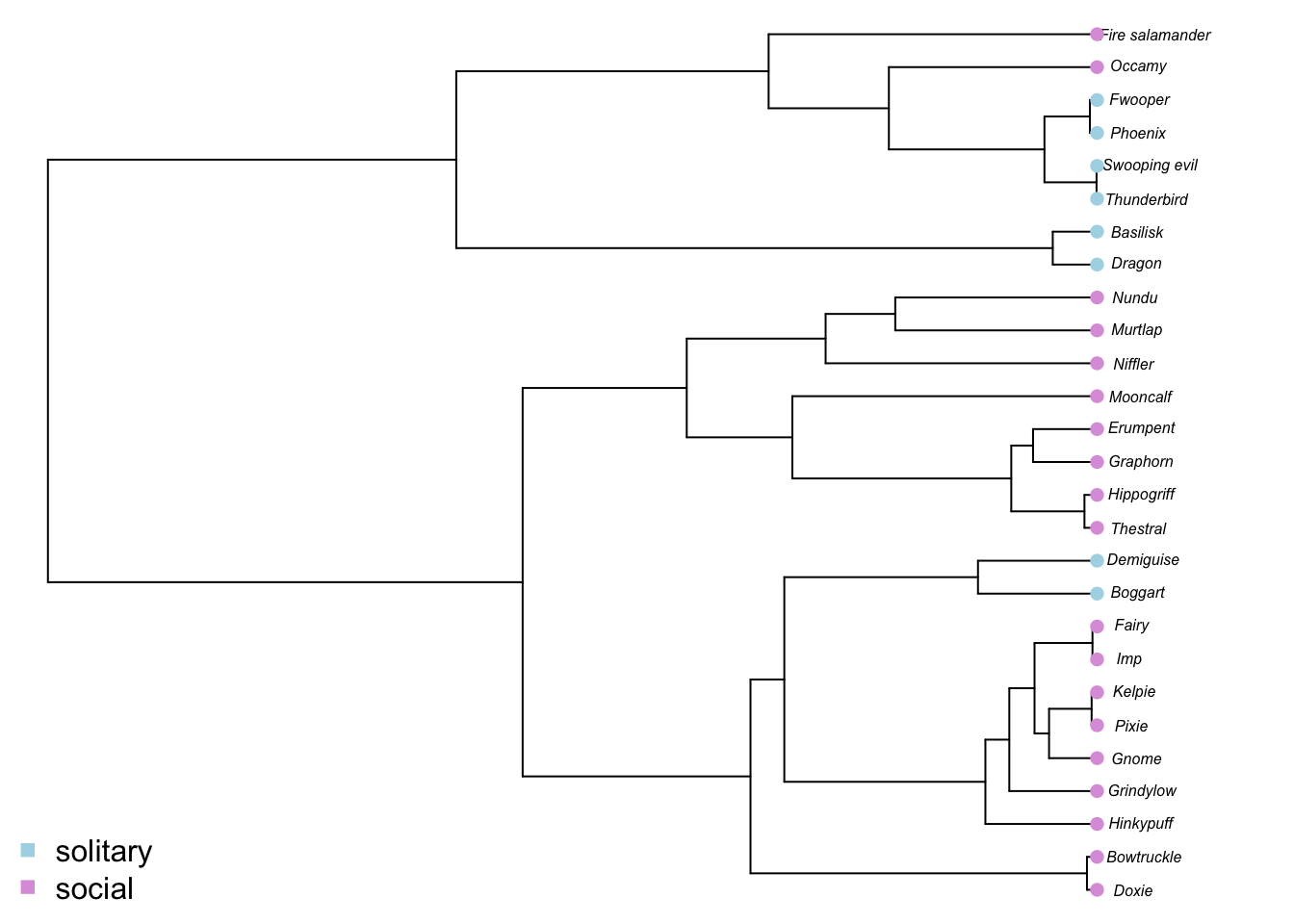

You’ll see that solitary behavior seems to be more restricted in its distribution. Most solitary magical creatures are bird or reptile like. From the distribution on the phylogeny, we might guess that solitary behavior is the ancestral state. This is exactly what we need to know in order to test whether evolutionary modes for body size vary for solitary vs social magical creatures. But before we can infer ancestral states, we need to chose the most appropriate model of social evolution.

There are several ways of mapping social status onto the tree but probably the most straightforward is to use an ancestral state estimation. We will estimate ancestral states for each node under a Markov model, pick the state with the highest marginal likelihood, and then assign that as the node state.

Unfortunately, just like rates can vary for continuous traits, so they can vary for discrete traits, and this can impact our ancestral state estimation. Fortunately, it’s straightforward to test for this kind of heterogeneity using the fitDiscrete function in the geiger package.

7.3 Models of discrete trait evolution

7.3.1 Mk1 – all rates equal (ER)

The simplest Markov model we can fit to comparative data is an Mk1 model – M for Markov, k1 for \(k = 1\) or 1 parameter. The single parameter of this model is a transition rate – the rate at which states change. Because we only have one rate, transitions between any pair of states occur at the same rate and are therefore equally probable. We can visualize the \(Q\) (rate) matrix for an Mk1 model like this:

-	1	2	3
1	-	1	1
2	1	-	1
3	1	1	-

The off-diagonals are the transition rates from state 1 to 2, 1 to 3, 2 to 1 and so on (read rows then columns). We typically designate individual transition rates in the form \(q_ij\), which means the rate of going from state \(i\) to state \(j\). Here, the 1 in all off-diagonal elements represents the fact that rates are the same regardless of what state \(i\) and \(j\) are, and the direction of that change. The diagonal elements \(q_ii\) give the rate of not changing and are computed as the negative sum of the non-diagonal row elements. This is so that the rows sum to zero.

If you’re familiar with models of molecular evolution, you might know this model better as the Jukes-Cantor model, where transition rates = transversion rates.

7.3.2 Mk – symmetric rates (SYM)

We could add some complexity, and perhaps realism, by imagining that the rate of change between any pair of states is the same regardless of direction, but that the rate of change differs among states. Such a model is referred to as a symmetric model, and has a \(Q\) matrix of the form:

-	1	2	3
1	-	1	2
2	1	-	3
3	2	3	-

Here, \(q_{12} = q_{21}\) but this rate is allowed to be different from \(q_{13}/q_{31}\) and from \(q_{23}/q_{32}\). The number of different rates is three for \(S = 3\). However, if we were to add a fourth state, the new number of rates would not be 4 but rather would be 6. This is because there would now be 6 distinct off-diagonal elements present in the upper or lower diagonals.

If you’re more familiar with molecular models, this is how we get the 6-rate GTR (General Time Reversible) model:

-	A	C	T	G
A	-	1	2	3
C	1	-	4	5
T	2	4	-	6
G	3	5	6	-

Obviously, a symmetric model with only 2 states becomes an equal rates (Mk1) model.

7.3.3 Mk – All Rates Different (ARD)

Finally, we can go crazy and allow all rates to be different. For S-states, this would generate \(S^2 - S\) rates which might be crazy, depending on how many states you have. For completeness, the \(Q\) matrix for an All Rates Different model would look like this:

-	1	2	3
1	-	1	2
2	3	-	4
3	5	6	-

If you’re more familiar with molecular models, then you’ll be aware that molecular folks don’t do this because of potential over-fitting. This is a very important point to consider. However, in comparative data, there are three situations in which this model might realistically be a good fit.

An All Rates Different model might be a good fit if you have an especially large datasets that spans a variety of different states. For example, if you had a tree of all 64,000 plus vertebrates and wanted to examine transition rates among different dietary strategies, this model would be worth examining.
If you have strong reasons to suppose character states are not reversible, this is worth using. For example, complex structures like eyes or teeth tend not to reappear once lost so asymmetric models might be a better fit for these kinds of characters.
This model is also a good option when you only have two states but think rates back and forth might be different. In this latter situation, the All Rates Different model simply gives you two rates, which isn’t really over-fitting.

7.4 Fitting the models using `fitDiscrete`

Let’s try these models with our magical creatures dataset using fitDiscrete. We will investigate rates of change in social status.

equal <- fitDiscrete(mytree, mydata[ , "SocialStatus"], model = "ER")
#sym <- fitDiscrete(mytree, mydata[ , "SocialStatus"], model = "SYM")
ard <- fitDiscrete(mytree, mydata[ , "SocialStatus"], model = "ARD")

Before moving on, note that the commented out fitting of the symmetric model is on purpose. Why? Remember that we only have 2 states, solitary and social. A symmetric model with 2 states is just an equal rates model, so we can conveniently ignore it here. Let’s look at the output for the equal rates model:

equal

## GEIGER-fitted comparative model of discrete data
##  fitted Q matrix:
##                  1            2
##     1 -0.002247321  0.002247321
##     2  0.002247321 -0.002247321
## 
##  model summary:
##  log-likelihood = -8.815776
##  AIC = 19.631552
##  AICc = 19.791552
##  free parameters = 1
## 
## Convergence diagnostics:
##  optimization iterations = 100
##  failed iterations = 0
##  frequency of best fit = 1.00
## 
##  object summary:
##  'lik' -- likelihood function
##  'bnd' -- bounds for likelihood search
##  'res' -- optimization iteration summary
##  'opt' -- maximum likelihood parameter estimates

This looks very similar to the output from fitContinuous. We’ve got a model summary, with log likelihoods and AIC scores, convergence diagnostics and an object summary. The only difference is the first part, which gives us a fitted \(Q\) matrix, rather than a summary of model parameters (the \(Q\) matrix is the model parameters). This is an equal rates model, so the two off-diagonal elements are all same, and the diagonals are the negative values of the rates (so rows sum to zero).

By typing ard, we can look at the output for the all-rates-different model:

ard

## GEIGER-fitted comparative model of discrete data
##  fitted Q matrix:
##                  1            2
##     1 -0.005617678  0.005617678
##     2  0.002368874 -0.002368874
## 
##  model summary:
##  log-likelihood = -8.634626
##  AIC = 21.269252
##  AICc = 21.769252
##  free parameters = 2
## 
## Convergence diagnostics:
##  optimization iterations = 100
##  failed iterations = 0
##  frequency of best fit = 0.38
## 
##  object summary:
##  'lik' -- likelihood function
##  'bnd' -- bounds for likelihood search
##  'res' -- optimization iteration summary
##  'opt' -- maximum likelihood parameter estimates

It seems as though the rate of moving from solitary to social (0.005) is slightly higher than the rate of going from social to solitary (0.002). Based on our color-coordinated plot from earlier, we might have predicted this to be the case.

Because the output of equal and ard are just like fitContinuous, we can pull AICc values out and use them to perform model selection:

aic.discrete <- setNames(c(equal$opt$aic, ard$opt$aic), c("equal", "different"))
weights <- aicw(aic.discrete)
weights

##                fit  delta         w
## equal     19.63155 0.0000 0.6939922
## different 21.26925 1.6377 0.3060078

Based on AIC weights, which model should we prefer?

The all-rates-different model is less strongly supported (AICcW = 0.306) than the equal rates model (AICcW = 0.694). Now we can move forward with reconstructing ancestral states under the preferred equal rates transition rate model.

7.5 Ancestral state reconstructions

Ancestral state reconstruction is probably one of the most over-used and uninformative methods in the phylogenetic comparative methods toolkit. There are many reasons to be highly skeptical of ancestral state estimates and interpretations of macroevolutionary patterns and process that are based on them. However, if you want to know if evolutionary tempo or mode have varied over clade history based on the state of a discrete trait, you’ll need to do it. We’ll use ape’s ace function here. There are other options out there, for example in the phytools package. But ace will work for our purposes.

To perform ancestral state estimation under the all-rates-different model:

asr <- ace(mydata[ , "SocialStatus"], mytree, type = "discrete", model = "ER")

You might see an error message appear saying NaNs produced.

Don’t worry about this – it happens when rates for one transition are particularly low but doesn’t really affect our node state estimates. One point to note here is that ace now defaults to a joint estimation procedure, where the ancestral states are optimized based on all information in the tree, not just the states at descendant tips.

We can access our ancestral states by typing:

asr$lik.anc

In this matrix, the columns correspond to nodes in the tree (the numbering is off, as we’ll see in a sec) and the two columns give the scaled likelihoods that the node is in states 1 or 2. The scaled likelihoods are like probabilities, so for the first node, we reconstruct state 1 with probability = 0.3 and state 2 with probability = 0.7 , but for node 2 the probability of state 1 = 0.05 while that of state 2 = 0.95. Scaled likelihoods lend themselves very well to graphical display, so we can visualize these states with pie charts on the tree we plotted earlier.

par(mar = c(0,0,0,0))
plot(mytree, cex = 0.5, adj = c(0.2))
nodelabels(pie = asr$lik.anc, piecol = social.colors, cex = 0.5)
tiplabels(pch = 16, col = social.colors[mydata[,"SocialStatus"]])
legend("bottomleft",legend=c("solitary", "social"), 
       pch = 15, col=c("lightblue", "plum"), bty = "n")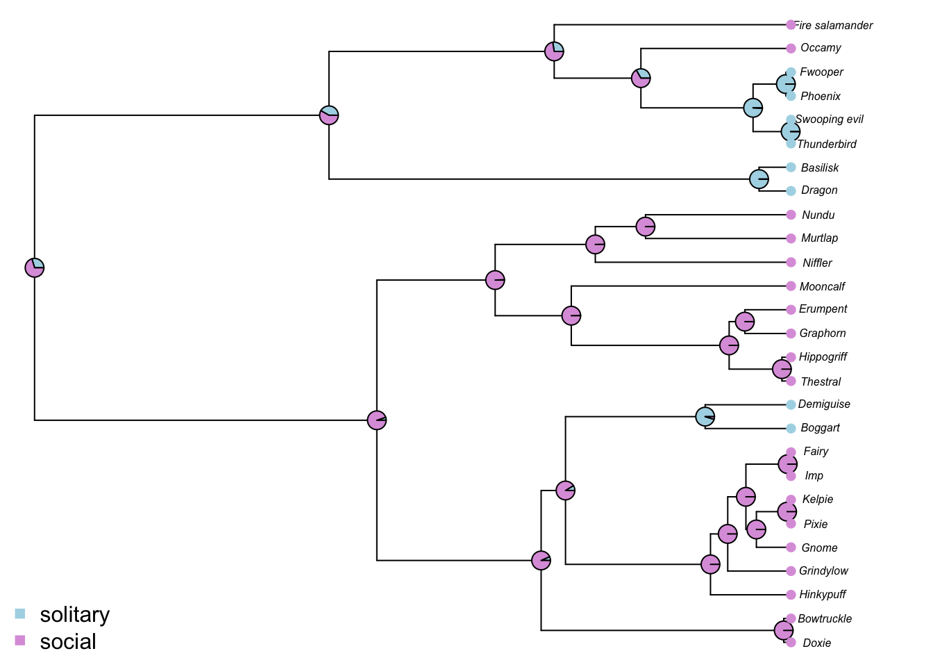

We reconstruct mostly social as the ancestral state for magical creatures, but with multiple transitions to solitary behaviour. For our next analyses though, we want to be able to extract the “best” state for each node. We can do this quite easily with the data structure ace gives us. First, we need to assign row names to our ancestral states that actual correspond to node numbers. phylo–format trees number nodes from n+1 onwards, where n is the number of taxa in the tree. So if there are 10 taxa, the root node is 11. Recall also that a fully bifurcating tree has n - 1 nodes. We can pull out the scaled likelihoods and number the rows appropriately with two simple lines of code:

node.states <- asr$lik.anc
rownames(node.states) <- seq(1:nrow(node.states)) + length(mytree$tip.label)
node.states

##               1            2
## 28 2.951598e-01 7.048402e-01
## 29 5.176500e-02 9.482350e-01
## 30 6.723783e-02 9.327622e-01
## 31 2.788813e-05 9.999721e-01
## 32 8.812542e-02 9.118746e-01
## 33 1.121960e-03 9.988780e-01
## 34 9.481369e-05 9.999052e-01
## 35 1.180908e-05 9.999882e-01
## 36 1.291077e-05 9.999871e-01
## 37 5.096106e-07 9.999995e-01
## 38 4.892579e-07 9.999995e-01
## 39 9.532305e-01 4.676946e-02
## 40 6.559008e-03 9.934410e-01
## 41 4.773548e-03 9.952265e-01
## 42 1.850043e-04 9.998150e-01
## 43 4.923981e-06 9.999951e-01
## 44 5.791449e-05 9.999421e-01
## 45 2.257465e-03 9.977425e-01
## 46 1.779187e-03 9.982208e-01
## 47 4.183958e-01 5.816042e-01
## 48 9.983242e-01 1.675751e-03
## 49 2.750360e-01 7.249640e-01
## 50 3.333531e-01 6.666469e-01
## 51 9.925342e-01 7.465840e-03
## 52 1.000000e+00 3.595570e-08
## 53 9.999929e-01 7.068412e-06

Now the rownumbers correspond to node numbers. This is useful. Now we’ll use a simple trick to extract the most likely states and assign them as node values on our tree.

best <- apply(node.states, 1, which.max)
best

## 28 29 30 31 32 33 34 35 36 37 38 39 40 41 42 43 44 45 46 47 48 49 50 51 52 
##  2  2  2  2  2  2  2  2  2  2  2  1  2  2  2  2  2  2  2  2  1  2  2  1  1 
## 53 
##  1

Now we have a named vector of “best” estimates of the node state. We can assign these to the tree using the following line of code.

mytree$node.label <- best
mytree

## 
## Phylogenetic tree with 27 tips and 26 internal nodes.
## 
## Tip labels:
##  Doxie, Bowtruckle, Hinkypuff, Grindylow, Gnome, Pixie, ...
## Node labels:
##  2, 2, 2, 2, 2, 2, ...
## 
## Rooted; includes branch lengths.

Now we have node labels associated with our magical tree that specify which social regime each branch is evolving under. We’re now ready to move on to modeling state specific rate variation and adaptive optima, using OUwie.

7.6 Fitting models using `OUwie`

OUwie (pronounced Ow-EE) is a package written by Brian O’Meara and Jeremy Beaulieu that performs maximum likelihood optimization of Brownian motion and Ornstein-Uhlenbeck models. The models implemented include the simple versions introduced earlier, but also include more complex versions that allow model parameters (rates, selection, optima) to vary among evolutionary regimes.

There are three things we need to fit an OUwie model. 1. A phylogeny with internal nodes labeled with the ancestral selective regimes - which we just did. 2. A dataset containing column entries in the following order: i) species names, ii) current selective regime, and iii) the continuous trait of interest. 3. The model we want to fit.

For the dataset all we need to do is make a dataframe with the relevant information. Let’s make it and look at the first few lines:

ouwie.data <- data.frame(species = rownames(mydata), regime = mydata[ , "SocialStatus"],
trait = log(mydata[ , "BodySize_kg"]))
# Look at the data
head(ouwie.data)

##               species regime      trait
## Doxie           Doxie      2  0.4054651
## Bowtruckle Bowtruckle      2 -1.0498221
## Hinkypuff   Hinkypuff      2  0.0000000
## Grindylow   Grindylow      2 -0.5978370
## Gnome           Gnome      2  3.2188758
## Pixie           Pixie      2 -0.9162907

Finally, we want to decide which model we’re going to fit.

7.6.1 Multi-rate Brownian motion (BMS)

In OUwie a multi-rate BM model is coded as “BMS”.

BMvariable <- OUwie(mytree, ouwie.data, model = "BMS")

## Initializing... 
## Finished. Begin thorough search... 
## Finished. Summarizing results.

Let’s look at the results:

BMvariable

## 
## Fit
##        lnL      AIC     AICc model ntax
##  -72.14716 152.2943 154.1125   BMS   27
## 
## Rates
##                 1          2
## alpha          NA         NA
## sigma.sq 7.269257 0.09645345
## 
## Optima
##                 1        2
## estimate 18.71153 2.902904
## se       65.09904 3.209815
## 
## Arrived at a reliable solution

The final line tells us that we arrived at a reliable solution – that is that the optimizer converged on a reliable set of parameter estimates. The rest of the output includes log likelihood (LnL), AIC (AIC) etc, the rates (including the alpha parameters), and the optima. There are three main things to notice:

You’ll see here that there are NAs for alpha because this is a BM model, so there is no \(\alpha\) parameter to estimate.
The optima here correspond to the root state for species with state 1 (solitary) or state 2 (social). It makes sense that the root state is higher for solitary species, as we know these can be huge (basilisks, dragons etc.) For OU models, these optima would be the adaptive optimal values of body mass for each of the two states.
The rates (sigma.sq) differ for regimes 1 and 2. Specifically, the rate for regime 1 (solitary) appears to be much higher that of regime 2 (social). So rates of body size evolution seem to be faster for solitary magical animals than for social magical animals, again this fits with our understanding of the data.

To know whether this difference is great enough for us to prefer this model, we’d need to compare AIC scores, or something similar. We’ll come back to this in a minute.

7.6.2 Multi-peak OU models

If you look at the help file for ?OUwie you’ll see the following options are available to us.

single-rate Brownian motion (model=BM1) [equivalent to “BM” in fitContinuous]
Brownian motion with different rate parameters for each state on a tree (model=BMS)
Ornstein-Uhlenbeck model with a single optimum for all species (model=OU1) [equivalent to “OU” in fitContinuous]
Ornstein-Uhlenbeck model with different state means and a single \(\alpha\) and \(\sigma^2\) acting on all selective regimes (model=OUM)
Ornstein-Uhlenbeck models that assume different state means as well as either multiple \(\sigma^2\) (model=OUMV), multiple \(\alpha\) (model=OUMA), or multiple \(\alpha\) and \(\sigma^2\) for each selective regime (model=OUMVA).

We have quite a few options when it comes to OU models; we can allow the optima to vary, the rates, the alphas and any combination of these. I’d encourage you to play around with these options with your own data, but for now, we’ll focus on the different optima models (OUM). Be aware too that these methods are very data hungry. I wouldn’t recommend fitting an OUMVA model to a tree with 50 tips – you’d need closer to 200 and ideally more to get good fits for this complex model. Of course here we only have 26 species so I wouldn’t trust these results (apart from the fact they are made up data about made up animals!).

OUmulti <- OUwie(mytree, ouwie.data, model = "OUM")

## Initializing... 
## Finished. Begin thorough search... 
## Finished. Summarizing results.

# Look at the results
OUmulti

## 
## Fit
##        lnL      AIC     AICc model ntax
##  -69.75334 147.5067 149.3249   OUM   27
## 
## 
## Rates
##                  1         2
## alpha     1.169449  1.169449
## sigma.sq 24.617820 24.617820
## 
## Optima
##                 1         2
## estimate 4.946723 2.5550174
## se       1.212267 0.7470149
## 
## Arrived at a reliable solution

What is different here?

We now have parameter estimates for alpha, as well as sigmasq. We can use the optima to infer an optimal size for solitary magical creatures of 4.947 log(body mass) units and an optimal mass of 2.555 log(body mass) units for social magical creatures. alpha is greater than zero suggesting that body size of magical creatures is evolving towards these optima.

To find out which model best fits our data, we’ll need to compute AIC weights again. Let’s compare these more complex models to the simple BM, EB and OU models we built in the first half of the practical. The code below will fit these in case you’ve started a new session.

BM <- fitContinuous(mytree, log(mydata[,"BodySize_kg"]), model = c("BM"))
OU <- fitContinuous(mytree, log(mydata[,"BodySize_kg"]), model = c("OU"))
EB <- fitContinuous(mytree, log(mydata[,"BodySize_kg"]), model = c("EB"))

aic.scores <- setNames(c(BM$opt$aicc, OU$opt$aicc, EB$opt$aicc, BMvariable$AICc, OUmulti$AICc), 
                       c("BM", "OU", "EB", "BMvariable", "OUmulti"))
aicw(aic.scores)

##                 fit     delta            w
## BM         201.5837 52.854229 1.841181e-12
## OU         148.7295  0.000000 5.523909e-01
## EB         204.1283 55.398776 5.158876e-13
## BMvariable 154.1125  5.383023 3.744018e-02
## OUmulti    149.3249  0.595374 4.101689e-01

Which is the best model overall?

7.7 References

Blomberg, S. P., T. Garland, and A. R. Ives. 2003. Testing for phylogenetic signal in comparative data: behavioral traits are more labile. Evolution 57:717–745.
Butler, M. A. and A. A. King. 2004. Phylogenetic comparative analysis: a modeling approach for adaptive evolution. The American Naturalist 164:683–695.
Cavalli-Sforza, L. L. and A. W. Edwards. 1967. Phylogenetic analysis. models and estimation procedures. American Journal of Human Genetics 19:233.
Cooper, N., R. P. Freckleton, and W. Jetz. 2011. Phylogenetic conservatism of environmental niches in mammals. Proceedings of the Royal Society B: Biological Sciences 278:2384–2391.
Cooper, N. and A. Purvis. 2010. Body size evolution in mammals: complexity in tempo and mode.The American Naturalist 175:727–738.
Cooper, N., Thomas, G.H., Venditti, C., Meade, A. & Freckleton, R.P. (2016b) A cautionary note on the use of ornstein-uhlenbeck models in macroevolutionary studies. Biological Journal of the Linnaean Society
Felsenstein, J. 1973. Maximum likelihood and minimum-steps methods for estimating evolutionary trees from data on discrete characters. Systematic Biology 22:240–249.
Freckleton, R. P. and P. H. Harvey. 2006. Detecting non-brownian trait evolution in adaptive radiations. PLoS Biology 4:e373.
Hansen, T. F. 1997. Stabilizing selection and the comparative analysis of adaptation. Evolution Pages 1341–1351.
Harmon, L. J., J. B. Losos, T. Jonathan Davies, R. G. Gillespie, J. L. Gittleman, W. Bryan Jennings, K. H. Kozak, M. A. McPeek, F. Moreno-Roark, T. J. Near, et al. 2010. Early bursts of body size and shape evolution are rare in comparative data. Evolution 64:2385–2396.
Lande, R. 1976. Natural selection and random genetic drift in phenotypic evolution. Evolution 30:314–334.
Slater, G. J., L. J. Harmon, and M. E. Alfaro. 2012. Integrating fossils with molecular phylogenies improves inference of trait evolution. Evolution 66:3931–3944.
Slater, G. J. and M.W. Pennell. 2014. Robust regression and posterior predictive simulation increase power to detect early bursts of trait evolution. Systematic Biology 63:293–308.