Ultimately, you want your neural network to generalize to “unseen data” so that it can be used in the real world. A neural network's ability to generalize to unseen data depends on two factors:
Your network is too simple to understand the training data’s salient features. This is called underfitting the training set.
Example: You train a 2-layer convolutional neural network on an ImageNet classification task (1000 classes that are very different from each other.)
Here’s a common trick to avoid underfitting: deepen your neural network by adding more layers.
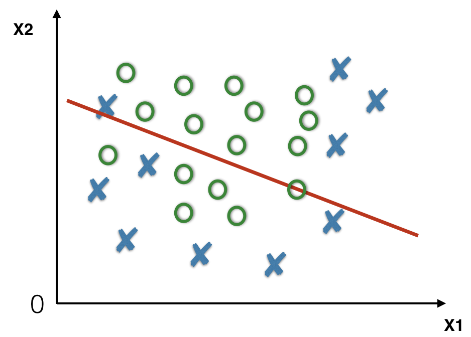
An underfit classifier will learn a simple decision boundary (red line) that fails to capture the structure of the training data resulting in many misclassified training points.
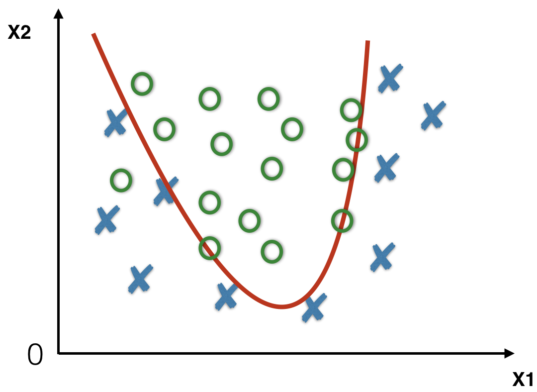
Your network is complex enough to fully memorize the mapping between the training data and the training labels. However, it does not generalize well to unseen data because it has merely over-memorized the salient features of the training set. This is called overfitting the training set.
Example 1: You train a 20-layer convolutional neural network to detect if there’s a cloud (label 1) or no clouds (label 0) in the sky.
Example 2: Consider a “day vs. night image classification”. Rather than understanding the inherent features of the data such as the brightness, the colors or the presence of a blue sky, your model learned mapping between training images and training labels by heart. You do not want this.
The best way to help your model generalize is to gather a larger dataset, but this is not always possible. When you do not have access to a large dataset, you can use regularization methods. Let’s learn the intuition behind these methods.
The number of parameter (weights) is usually a proxy to measure the complexity of a network.
An overfit classifier will learn a complex decision boundary (red line) that correctly classifies most of the training data, but will not generalize to unseen data.
What are the hints telling us that the image was taken during the day or the night?
Before we explore the main regularization methods, you must partition your dataset. In order to estimate the ability of your model to generalize, you will split your dataset into three (or sometimes more) sets: training, dev and test. If your model is trained on the training set, tuned on the dev set, and still performs well on the test set, it is able to generalize successfully.
| Train Accuracy | Dev Accuracy | Test Accuracy | Conclusion |
|---|---|---|---|
| 99% | 75% | 70% | Overfitting (high variance) |
| 88% | 85% | 83% | Underfitting (high bias) |
| 95% | 93% | 92% | Appropriate (correct bias/variance trade-off) |
You want to close the performance gap between your test set and your dev and training set while keeping the training performance as high as possible. Let’s delve into the methods that will help you do so.
The data used to train your model.
The data used to tune the hyperparameters of your model. This is sometimes referred to as a "validation" set.
The data used to evaluate the performance of your model in real life.
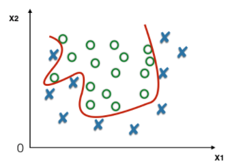
An appropriate classifier will learn a decision boundary (red line) that correctly classifies most of the training data, and will generalize to unseen data.
One of the widely used regularization method is called early stopping. Recall that optimizing a network to find the correct parameters is an iterative process. If you evaluate your model’s error on the training and dev set after every training epoch, you might see such curves:
Based on this observation, you can estimate that after the 30,000th epoch, your model starts overfitting to the training set. Early stopping means saving the model’s parameters at the 30,000th epoch. The saved model is the best performing model on the dev set and will likely generalize better to the test set.
Examples of optimizations are Stochastic Gradient Descent, Adam, Momentum or RMS Prop.
An epoch is one optimization pass over the entire dataset. In full-batch gradient descent, one epoch is one iteration, but in stochastic gradient descent, one epoch is multiple iterations.
def early_stopping(model, X_train, Y_train, X_dev, Y_dev, eval_freq = 1, stop_wait = 100):
    """
    Python implementation of the early stopping algorithm.

    Arguments:
    model -- Your model class which comes with functions:
                model.train() -- trains the model for one step and returns the updated model.
                model.eval() -- evaluates the model on a set and returns the error.
                model.copy() -- copies the model.
    X_train -- Training set
    Y_train -- Training labels
    X_dev -- Dev set
    Y_dev -- Dev labels
    eval_freq -- integer, ratio of training step per evaluation step.
    stop_wait -- number of train step without dev error improvement before stopping.

    Returns:
    best_model -- the model with minimal dev error and early stopping
    best_dev_error -- the best dev error achieved by best_model
    best_model_index -- the best_model's saving step
    """

    current_model = model.copy()       # Track your current model
    best_model = model.copy()          # Track your best model
    num_train_steps = 0                # number of training steps
    num_steps_since_best_model = 0     # number of training steps since the last best model was saved
    best_dev_error = np.inf            # the best dev error achieved so far (by best_model)
    best_model_index = 0               # the best_model's saving step

    # Loop unless there's no model improvement on the dev set for stop_wait steps.
    while num_steps_since_best_model < stop_wait:

        # Train current_model for "train_per_eval_ratio" steps
        for s in range(train_per_eval_ratio):
            current_model.train(X_train, Y_train)
            num_train_steps = num_train_steps + 1

        # Evaluate your current_model on the dev set.
        dev_error = current_model.eval(X_dev, Y_dev)

        # If the dev error is lower than the best dev error previously achieved, then save the current_model as the best_model
        if dev_error < best_dev_error:
            num_steps_since_best_model = 0
            best_model = current_model.copy()
            best_model_index = num_train_steps
            current_model = best_model
        # Otherwise increment num_steps_since_best_model
        else:
            num_steps_since_best_model = num_steps_since_best_model + 1

        return best_model, best_dev_error, best_model_index
Despite being practical, early stopping is not satisfying from a scientific standpoint. There exist other regularization methods, such as L1 (/L2) regularization and dropout, or optimization methods, such as learning rate annealing, that rely more on theory and are often more reliable.
In order to avoid overfitting the training set, you can try to reduce the complexity of the model by removing layers, and consequently decreasing the number of parameters. As shown by the work of Krogh and Hertz (1992), another way to constrain a network and lower its complexity is to:
Limit the growth of the weights through some kind of weight decay.
You want to prevent the weights from growing too large, unless it is really necessary. Intuitively, you are reducing the set of potential networks to choose from.
L1 and L2 regularizations can be achieved by simply adding a term that penalizes large weights to the cost function. If you were training a network to minimize the cost with (let’s say) gradient descent, your weight update rule would be:
Instead, you would now train a network to minimize the cost where and . Your weight update rule would be:
For L1 regularization, this would lead to the update rule:
For L2 regularization, this would lead to the update rule:
At every step of L1 and L2 regularization the weight is pushed to a slightly lower value because , causing weight decay.
In statistics, a linear regression with L1 regularization is sometimes referred to as Lasso regression.
In statistics, a linear regression with L2 regularization is sometimes referred to as Ridge regression.
The update rules are different. While the L2 “weight decay” penalty is proportional to the value of the weight to be updated, the L1 “weight decay” is not.
For L2, the smaller the , the smaller the penalty during the update of and vice-versa for larger .
For L1, the penalty is independent of the value of , but the direction of the penalty (positive or negative) depends on the sign of . This results in an effect called “feature selection” or “weight sparsity”. L1 regularization makes the non-relevant weights 0.
You can play with the visualization below to see the impact of L1 and L2 regularization on the weights during training.
As you can see, L1 and L2 regularizations have a dramatic effect on the weights values:
For the L1 regularization:The weight sparsity effect caused by L1 regularization makes your model more compact in theory, and leads to storage-efficient compact models that are commonly used in smart mobile devices.
Deep learning frameworks such as Keras allow you to add L1 or L2 regularization to your network in one line of code. The difference in the optimization process is implemented automatically. Here's an example: L1 and L2 regularization in Keras.
It’s useful to build some intuition about what L1 and L2 regularization do. You can play with the visualization below to observe variations of the cost landscape subject to regularization from a top view.
As you can see, L1 and L2 regularizations have a dramatic effect on the geometry of the cost function:
Although L1 and L2 regularization are simple techniques to reducing overfitting, there exist other methods, such as dropout regularization, that have been shown to be more effective at regularizing larger and more complex networks. If you had unlimited computational power, you could improve generalization by averaging the predictions of several different neural networks trained on the same task. The combination of these models will likely perform better than a single neural network trained on this task. However, with deep neural networks, training various architectures is expensive because:
Dropout is a regularization technique, introduced in Srivastava et al. (2014), that allows you to combine many different architectures efficiently by randomly dropping some of the neurons of your network during training.
Dropout is discussed in detail in our Deep Learning Specialization (Course 2: “Improving Neural Networks”, Week 2: “Practical aspects of Deep Learning”). We invite you to check it out to understand the intuition behind dropout.
This, in fact, is the motivation behind ensemble methods such as random forest.
When applying regularization methods, you need a metric to track your model's improvement and generalization ability. The bias/variance tradeoff enables you to measure the efficiency of your regularization.
The bias/variance tradeoff is discussed in our Deep Learning Specialization (Course 2: “Improving Neural Networks”, Week 2: “Practical aspects of Deep Learning”). We invite you to check it out!
Successfully training a model on complex tasks is complicated. You need to find a model architecture that can encompass the complexity of the dataset. Once you find such an architecture, you can work on improving generalization. Exploring, and even combining, different regularization techniques is an unmissable step of the training process. It helps you build intuition on the ability of a model to generalize in the real-world.
↑ Back to top