Optimization

Training a machine learning model is a matter of closing the gap between the model's predictions and reality. But optimizing the model isn't so straightforward. Through interactive visualizations, we'll help you develop your intuition for setting up and solving the optimization problem.

Table of content

Setting up the optimization problem
Running the optimization process

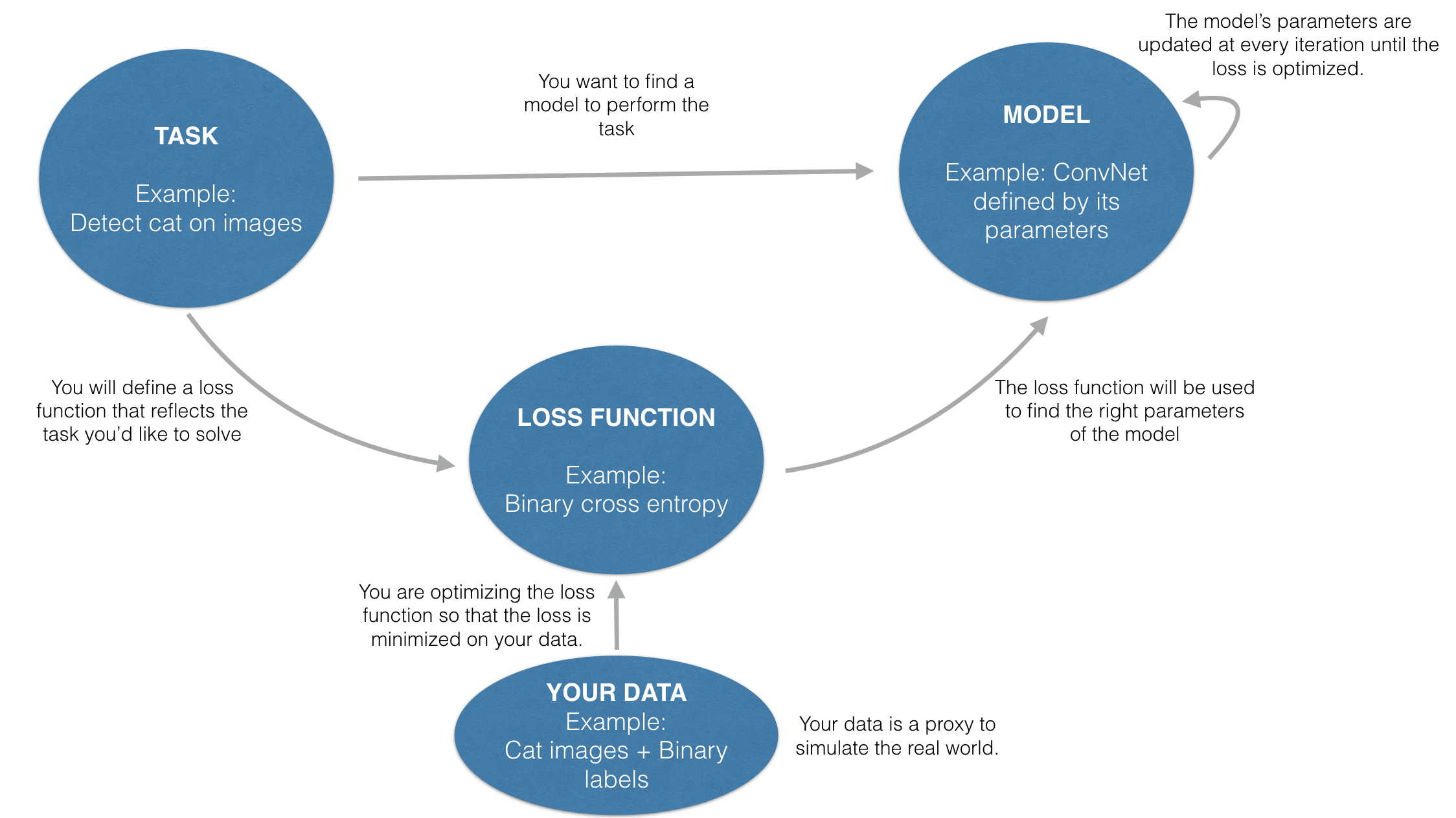
In machine learning, you start by defining a task and a model consisting of an architecture and parameters. For a given architecture, the values of the parameters determine how accurately the model performs the task. But how do you find good values? By defining a loss function that evaluates how well the model performs. The goal is to optimize the loss function and thereby to find parameter values that close the gap between the model's predictions and reality.

I Setting up the optimization problem

The loss function will be different in different tasks depending on the output desired. How you define it has a major influence on how the model will train and perform. Let's consider two examples:

Example 1: House price prediction

Say your task is to predict the price of houses based on features such as floor area, number of bedrooms, and ceiling height. The loss function can be summarized by the sentence:

Given a set of house features, the square of the difference between your prediction and the actual price should be as small as possible.

You define the loss function as

where is your predicted price and is the actual price, also known as ground truth.

Example 2: object detection

Let's consider a more complex example. Say your task is to detect (that is, localize and identify) cars and pedestrians in images. The loss function should frame the following sentence in mathematical terms:

Given an image, predict bounding boxes (bbox) that contain all the cars and pedestrians in the image. The predicted boxes should match the size, position and class of the actual objects.

In mathematical terms, a possible loss function (Redmon et al., 2016) is:

This loss function depends on:

Parameters of the network (weights and biases)
Input to the network (images)
Ground truth corresponding to the input (labels comprising bounding boxes and classes)

For a fixed value of the input batch and ground-truth batch, the loss has a landscape that depends on the parameters of the network. It is difficult to visualize the loss landscape (against the parameters) if there are more than two parameters. However, the landscape does exist and our goal is to find the point where the loss value is minimal. Updating the parameter values will move the loss value either closer to or farther from the target minimum point.

By definition, this function L has a low value when the model performs well on the task.

The relationship between the model and the loss function

It is important to distinguish between the function that will perform the task (the model) and the function you are optimizing (the loss function).

The model is an architecture and a set of parameters that approximates a real function that performs the task. The optimized parameter values will enable the model to perform the task with relative accuracy.
The loss function quantifies how accurately the model performs on given data set. Its value depends on the model's parameter values.

At this point, good parameter values are unknown. However, you have a formula for the loss function. Optimize that, and you will find good parameter values. The way to do this is to feed the training data set into the model, find the loss function, and adjust the parameters to make it as small as possible. This is usually an iterative process.

In summary, the way you define the loss function will dictate the performance of your model on the task at hand. The diagram below illustrates the process of finding a model that performs the task at hand.

Do you know the mathematical formula that allows you to detect cats in images? Probably not, but using data you can find a function that performs this task. It turns out that a convolutional architecture with the right parameters defines a function that can perform this task well.

II Running the optimization process

In this section, assume that you have already chosen a task and a loss function. You will minimize the loss function to find good parameter values.

Initialization, learning rate, and batch size

First, initialize the parameters so you have a starting point for optimization. You also need to choose hyperparameters such as learning rate and batch size. They will have an important influence on the optimization.

In the visualization below, you can play with the starting point of initialization, learning rate, and batch size. With these parameters, you will fit a linear regression on a set of 300 data points using the gradient descent optimization algorithm. For more information on gradient descent optimization, see the Deep Learning Specialization (Course 1: Neural Networks and Deep Learning, Week 2: Logistic Regression as a Neural Network.) Here are some questions to ask yourself:

Why does the loss landscape look like this?
What is the red dot?
Why can your optimization end up with a cost value lower than the ground truth line?
What is the impact of the learning rate on the optimization?
What is the impact of the batch size on the optimization?

1. Generate your dataset

Select a training set size.

Small Medium Large

A training set of the chosen size will be sampled with noise from a "ground truth" line. This line is the target line for your network function defined by .

2. Observe the loss landscape and initialize parameters

The loss function is the L2 loss defined as . The blue dot indicates the value of the loss function at the "ground truth" slope and intercept. The red dot indicates the value of the loss function at a chosen initialization of the slope and intercept. Drag and drop the red dot to change the initialization.

3. Optimize your loss function

You can now iteratively update your parameters to minimize the loss. Select a learning rate.

Small Medium Large

Select a batch size to use.

Stochastic Mini-batch Full-batch

Train your network function.

Here are some takeaways from the visualization:

a) Initialization

A good initialization can make your optimization quicker and converge to the correct minimum (in the case where there are several minima). If you want to learn more about initialization, read our AI Note on Initializing neural networks.

b) Learning rate

The choice of learning rate influences the convergence of your optimization.

If the learning rate is too small, your updates are small and the optimization is slow. Furthermore, you’re likely to settle into an inappropriate local minimum. (We use this term because, in machine learning optimization, the optimization is often non-convex and unlikely to converge to the global minimum.)
If the learning rate is too large, your updates will be large and the optimization is likely to diverge.
If the learning rate is appropriate, your updates are appropriate and the optimization will converge.

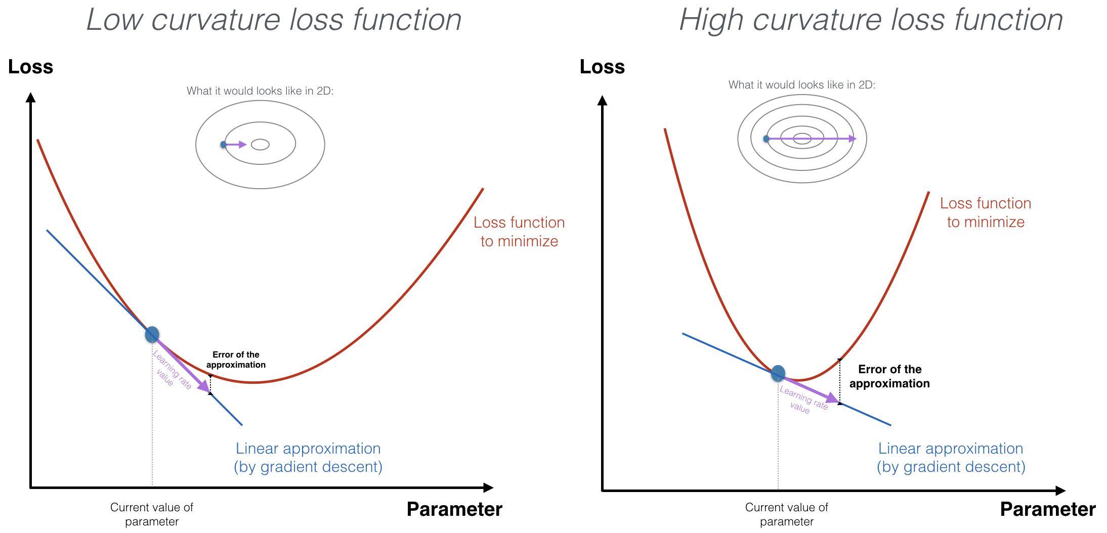
The choice of learning rate depends on the curvature of your loss function. Gradient descent makes a linear approximation of the loss function in a given point. It then moves downhill along the approximation of the loss function. In the case where the loss is highly curved, the larger your step size (learning rate), the larger the error of your approximation. Taking small steps reduces the error¹.

It is common practice to start with a large learning rate and decay it during training. Choosing the right decay (how often? by how much?) is non-trivial. An excessively aggressive decay schedule slows the progress towards the optimum, while a slow-paced decay schedule leads to chaotic updates with small improvements.

Here we say inappropriate local minimum because in machine learning optimization, the optimzation is often non-convex and unlikely to converge to the global minimum.

c) Batch size

The right choice of batch size is crucial to ensure convergence and generalization of your network. Although there’s been some research² on how to choose the batch size, there’s no consensus yet on what batch size to choose. In practice, you can use a hyperparameter search to choose a good batch size.

Recent research into batch size has uncovered the following principles:

The batch size determines the frequency of your updates. The smaller the batches, the more — though quicker — the updates.
The larger the batch size, the more accurate the gradient of the loss will be with respect to the parameters. That is, the direction of the update is most likely going down the local slope of the loss landscape.
Choosing the largest batch size that fits in GPU memory results in efficient parallelization and usually accelerates training.
However, large batch sizes can sometimes hurt the ability to generalize.

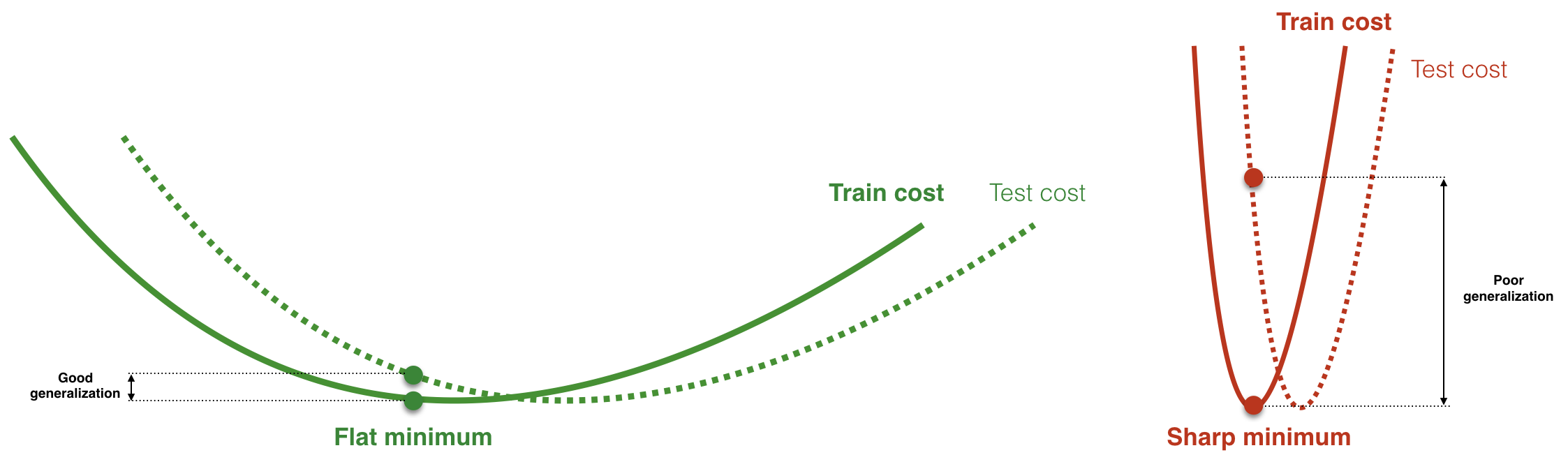
In choosing batch size, there’s a balance to be struck depending on the task you’re trying to achieve. Recall that the input batch is an input to the cost function. Large batch size typically leads to sharper cost function surfaces than a small batch size, as Keskar et al. find in their paper, On large-batch training for deep learning: generalization gap and sharp minima. Here's a figure comparing a flat and a sharp minumum. Flat cost surfaces (and thus small batche sizes) are preferred because they lead to good generalization without requiring high precision.

In practice, to find hyperparameters such as learning rate and batch size, you should perform hyperparameter search. Batch size and learning rate are two ways to achieve the same outcome, according to Smith, Kindermans et al. in Don't Decay the Learning Rate, Increase the Batch Size. They argue that the benefits of decaying the learning rate can be achieved by increasing batch size during training. So if you change batch size, you may also need to change learning rate. The efficient use of vast batch sizes notably reduces the number of parameter updates required to train a model.

d) Iterative update

Now that you have a starting point, a learning rate, and a batch size, it’s time to iteratively update the parameters to move toward the minimum of the loss function.

The optimization algorithm is also a core choice. You can play with various optimizers in the visualization below. That will help you build intuition regarding the pros and cons of each.

In this visualization, you will choose the loss function and the starting point of your optimization. Although there's no explicit network function, you can assume that finding the minimum of your loss function is equivalent to finding the best network function for your task.

1. Choose a loss landscape

Select an artificial landscape .

2. Choose initial parameters

On the loss landscape graph, drag the red dot to choose the initial parameters values and thus the initial value of the loss.

3. Choose an optimizer

Select the optimizer and its hyperparameters.

Optimizer	Learning Rate	Learning Rate Decay
Gradient Descent
Momentum
RMSprop
Adam

Optimize your loss function.

This 2D plot describes the value of your loss function for different values of the 2 parameters . The darker the color, the larger the loss value.

The choice of optimizer influences both the speed of convergence and whether it occurs. Several alternatives to the classic gradient descent algorithms have been developed in the past few years and are listed in the table below. (Notation: )

Optimizer	Update rule	Attribute
(Stochastic) Gradient Descent		GD can use parallelization efficiently, but is very slow when the data set is larger the GPU's memory can handle. The parallelization wouldn't be optimal. SGD usually converges faster than GD on large datasets, because updates are more frequent. Plus, the stochastic approximation of the gradient is usually precise without using the whole dataset because the data is often redundant. Of the optimizers profiled here, SGD uses the least memory for a given batch size.
Momentum		Momentum speeds up the learning with a very minor implementation change. Momentum uses more memory for a given batch size than SGD but less than RMSprop and Adam.
RMSprop		RMSprop’s adaptive learning rate prevents the learning rate decay from diminishing too slowly or too fast. RMSprop maintains per-parameter learning rates. RMSprop usually works well in online and non-stationary settings. RMSprop uses more memory for a given batch size than SGD and Momentum, but less than Adam.
Adam		The hyperparameters of Adam (learning rate, exponential decay rates for the moment estimates, etc.) are usually set to predefined values (given in the paper), and do not need to be tuned. Adam performs a form of learning rate annealing with adaptive step-sizes. Of the optimizers profiled here, Adam uses the most memory for a given batch size. Adam is often the default optimizer in machine learning.

Online optimization is when updates must be made with incomplete knowledge of the future (as in Stochastic Gradient Descent optimization).

Non-stationary setting essentially describes inflection points (where the concavity of the landscape changes) for which the gradient is zero in some, but not all, directions.

Despite performing well in the initial portion of training, adaptive optimization methods such as Adam or RMSprop have been found to generalize poorly at later stages of training compared to Stochastic Gradient Descent (SGD). In Improving Generalization Performance by Switching from Adam to SGD, Keskar et al. investigate a hybrid strategy that begins training with an adaptive method and switches to SGD when appropriate.

You can find more information about these optimizers in the Deep Learning Specialization (Course 2: Improving your Deep Neural Network, Week 2: Optimization) on Coursera.

Conclusion

Exploring the optimization methods and hyperparameters presented above can help you build intuition for optimizing networks for your own tasks. Intuitively understanding the sensitivity of the loss optimization for these hyperparameters (learning rate, batch size, optimizer, and so on) is important during hyperparameter search. Combined with the right method (random search or Bayesian optimization), it will help you iterate through your search to find the right model.

Optimizing neural networks