6 Other functionalities
The dispRity package also contains several other functions that are not specific to multidimensional analysis but that are often used by dispRity internal functions.
However, we decided to make these functions also available at a user level since they can be handy for certain specific operations!
You’ll find a brief description of each of them (alphabetically) here:
6.1 char.diff
This is yet another function for calculating distance matrices.
There are many functions for calculating pairwise distance matrices in R (stats::dist, vegan::vegdist, cluster::daisy or Claddis::calculate_morphological_distances) but this one is the dispRity one.
It is slightly different to the ones mentioned above (though not that dissimilar from Claddis::calculate_morphological_distances) in the fact that it focuses on comparing discrete morphological characters and tries to solve all the problems linked to these kind of matrices (especially dealing with special tokens).
The function intakes a matrix with either numeric or integer (NA included) or matrices with character that are indeed integers (e.g."0" and "1").
It then uses a bitwise operations architecture implemented in C that renders the function pretty fast and pretty modular.
This bitwise operations translates the character states into binary values.
This way, 0 becomes 1, 1 becomes 2, 2 becomes 4, 3 becomes 8, etc…
Specifically it can handle any rules specific to special tokens (i.e. symbols) for discrete morphological characters. For example, should you treat missing values "?" as NA (ignoring them) or as any possible character state (e.g. c("0", "1")?)? And how to treat characters with a ampersand ("&")? char.diff can answer to all these questions!
Let’s start by a basic binary matrix 4*3 with random integer:
## A random binary matrix
matrix_binary <- matrix(sample(c(0,1), 12, replace = TRUE), ncol = 4,
                        dimnames = list(letters[1:3], LETTERS[1:4]))
By default, char.diff measures the hamming distance between characters:
##   A B C D
## A 0 0 1 1
## B 0 0 1 1
## C 1 1 0 0
## D 1 1 0 0
## attr(,"class")
## [1] "matrix"    "char.diff"
Note that the results is just a pairwise distance (dissimilarity) matrix with some special dual class matrix and char.diff.
This means it can easily be plotted via the disparity package:

You can check all the numerous plotting options in the ?plot.char.diff manual (it won’t be developed here).
The char.diff function has much more options however (see all of them in the ?char.diff manual) for example to measure different differences (via method) or making the comparison work per row (for a distance matrix between the rows):
##          a        b        c
## a 0.000000 1.414214 1.414214
## b 1.414214 0.000000 0.000000
## c 1.414214 0.000000 0.000000
## attr(,"class")
## [1] "matrix"    "char.diff"
We can however make it more interesting by playing with the different rules to play with different tokens.
First let’s create a matrix with morphological characters as numeric characters:
## A random character matrix
(matrix_character <- matrix(sample(c("0","1","2"), 30, replace = TRUE), ncol = 5,
                           dimnames = list(letters[1:6], LETTERS[1:5])))
## A B C D E
## a "1" "1" "1" "1" "0"
## b "0" "2" "0" "2" "0"
## c "2" "2" "1" "2" "0"
## d "1" "2" "0" "0" "1"
## e "2" "2" "1" "1" "2"
## f "0" "2" "0" "2" "0"## A B C D E
## A 0.0 0.6 0.6 0.6 0.8
## B 0.6 0.0 0.4 0.4 0.8
## C 0.6 0.4 0.0 0.4 0.6
## D 0.6 0.4 0.4 0.0 1.0
## E 0.8 0.8 0.6 1.0 0.0
## attr(,"class")
## [1] "matrix" "char.diff"Here the characters are automatically converted into bitwise integers to be compared efficiently. We can now add some more special tokens like "?" or "0/1" for uncertainties between state "0" and "1" but not "2":
## Adding uncertain characters
matrix_character[sample(1:30, 8)] <- "0/1"

## Adding missing data
matrix_character[sample(1:30, 5)] <- "?"

## This is what it looks like now
matrix_character
## A B C D E
## a "?" "?" "1" "1" "0"
## b "0" "0/1" "0/1" "0/1" "0"
## c "2" "2" "?" "0/1" "0"
## d "1" "2" "0" "0/1" "1"
## e "?" "2" "1" "1" "2"
## f "0" "2" "0" "?" "0/1"## The hamming difference between columns including the special characters
char.diff(matrix_character)## A B C D E
## A 0.0000000 0.6666667 1.00 0.50 0.6666667
## B 0.6666667 0.0000000 1.00 1.00 0.7500000
## C 1.0000000 1.0000000 0.00 0.00 0.2500000
## D 0.5000000 1.0000000 0.00 0.00 0.2500000
## E 0.6666667 0.7500000 0.25 0.25 0.0000000
## attr(,"class")
## [1] "matrix" "char.diff"Note here that it detected the default behaviours for the special tokens "?" and "/": "?" are treated as NA (not compared) and "/" are treated as both states (e.g. "0/1" is treated as "0" and as "1").
We can specify both the special tokens and the special behaviours to consider via special.tokens and special.behaviours.
The special.tokens are missing = "?", inapplicable = "-", uncertainty = "\" and polymorphism = "&" meaning we don’t have to modify them for now.
However, say we want to change the behaviour for "?" and treat them as all possible characters and treat "/" as only the character "0" (as an integer) we can specify them giving a behaviour function:
## Specifying some special behaviours
my_special_behaviours <- list(missing = function(x,y) return(y),
                              uncertainty = function(x,y) return(as.integer(0)))

## Passing these special behaviours to the char.diff function
char.diff(matrix_character, special.behaviour = my_special_behaviours)
## A B C D E
## A 0.0 0.6 0.6 0.6 0.6
## B 0.6 0.0 0.8 0.8 0.8
## C 0.6 0.8 0.0 0.4 0.6
## D 0.6 0.8 0.4 0.0 1.0
## E 0.6 0.8 0.6 1.0 0.0
## attr(,"class")
## [1] "matrix" "char.diff"The results are quiet different as before! Note that you can also specify some really specific behaviours for any type of special token.
## Adding weird tokens to the matrix
matrix_character[sample(1:30, 8)] <- "%"

## Specify the new token and the new behaviour
char.diff(matrix_character, special.tokens = c(weird_one = "%"),
                            special.behaviours = list(
                                weird_one = function(x,y) return(as.integer(42)))
                            )
## A B C D E
## A 0 1 1 0 NaN
## B 1 0 1 1 NaN
## C 1 1 0 0 0
## D 0 1 0 0 0
## E NaN NaN 0 0 0
## attr(,"class")
## [1] "matrix" "char.diff"Of course the results can be quiet surprising then… But that’s the essence of the modularity. You can see more options in the function manual ?char.diff!
6.2 clean.data
This is a rather useful function that allows matching a matrix or a data.frame to a tree (phylo) or a distribution of trees (multiPhylo).
This function outputs the cleaned data and trees (if cleaning was needed) and a list of dropped rows and tips.
## Generating a trees with labels from a to e
dummy_tree <- rtree(5, tip.label = LETTERS[1:5])

## Generating a matrix with rows from b to f
dummy_data <- matrix(1, 5, 2, dimnames = list(LETTERS[2:6], c("var1", "var2")))

##Cleaning the trees and the data
(cleaned <- clean.data(data = dummy_data, tree = dummy_tree))
## $tree
##
## Phylogenetic tree with 4 tips and 3 internal nodes.
##
## Tip labels:
## D, B, E, C
##
## Rooted; includes branch lengths.
##
## $data
## var1 var2
## B 1 1
## C 1 1
## D 1 1
## E 1 1
##
## $dropped_tips
## [1] "A"
##
## $dropped_rows
## [1] "F"6.3 crown.stem
This function quiet handily separates tips from a phylogeny between crown members (the living taxa and their descendants) and their stem members (the fossil taxa without any living relatives).
data(BeckLee_tree)
## Diving both crow and stem species
(crown.stem(BeckLee_tree, inc.nodes = FALSE))
## $crown
## [1] "Dasypodidae" "Bradypus" "Myrmecophagidae" "Todralestes"
## [5] "Potamogalinae" "Dilambdogale" "Widanelfarasia" "Rhynchocyon"
## [9] "Procavia" "Moeritherium" "Pezosiren" "Trichechus"
## [13] "Tribosphenomys" "Paramys" "Rhombomylus" "Gomphos"
## [17] "Mimotona" "Cynocephalus" "Purgatorius" "Plesiadapis"
## [21] "Notharctus" "Adapis" "Patriomanis" "Protictis"
## [25] "Vulpavus" "Miacis" "Icaronycteris" "Soricidae"
## [29] "Solenodon" "Eoryctes"
##
## $stem
## [1] "Daulestes" "Bulaklestes" "Uchkudukodon"
## [4] "Kennalestes" "Asioryctes" "Ukhaatherium"
## [7] "Cimolestes" "unnamed_cimolestid" "Maelestes"
## [10] "Batodon" "Kulbeckia" "Zhangolestes"
## [13] "unnamed_zalambdalestid" "Zalambdalestes" "Barunlestes"
## [16] "Gypsonictops" "Leptictis" "Oxyclaenus"
## [19] "Protungulatum" "Oxyprimus"Note that it is possible to include or exclude nodes from the output. To see a more applied example: this function is used in chapter 03: specific tutorials.
6.4 get.bin.ages
This function is similar than the crown.stem one as it is based on a tree but this one outputs the stratigraphic bins ages that the tree is covering.
This can be useful to generate precise bin ages for the chrono.subsets function:
##  [1] 132.9000 129.4000 125.0000 113.0000 100.5000  93.9000  89.8000  86.3000
##  [9]  83.6000  72.1000  66.0000  61.6000  59.2000  56.0000  47.8000  41.2000
## [17]  37.8000  33.9000  28.1000  23.0300  20.4400  15.9700  13.8200  11.6300
## [25]   7.2460   5.3330   3.6000   2.5800   1.8000   0.7810   0.1260   0.0117
## [33]   0.0000
Note that this function outputs the stratigraphic age limits by default but this can be customisable by specifying the type of data (e.g. type = "Eon" for eons).
The function also intakes several optional arguments such as whether to output the startm end, range or midpoint of the stratigraphy or the year of reference of the International Commission of Stratigraphy.
To see a more applied example: this function is used in chapter 03: specific tutorials.
6.5 match.tip.edge
This function matches a vector of discreet tip values with the edges connecting these tips in the "phylo" structure.
This can be used to pull the branches of interest for some specific trait of some group of species or for colouring tree tips based on clades.
For example, with the charadriiformes dataset, you can plot the tree with the branches coloured by clade.
To work properly, the function requires the characteristics of the tip labels (e.g. the clade colour) to match the order of the tips in the tree:
## Loading the charadriiformes data
data(charadriiformes)
## Extracting the tree
my_tree <- charadriiformes$tree
## Extracting the data column that contains the clade assignments
my_data <- charadriiformes$data[, "clade"]
## Changing the levels names (the clade names) to colours
levels(my_data) <- c("orange", "blue", "darkgreen")
my_data <- as.character(my_data)
## Matching the data rownames to the tip order in the tree
my_data <- my_data[match(ladderize(my_tree)$tip.label, rownames(charadriiformes$data))]
We can then match this tip data to their common descending edges.
We will also colour the edges that is not descendant directly from a common coloured tip in grey using "replace.na = "grey".
Note that these edges are usually the edges at the root of the tree that are the descendant edges from multiple clades.
## Matching the tip colours (labels) to their descending edges in the tree
## (and making the non-match edges grey)
clade_edges <- match.tip.edge(my_data, my_tree, replace.na = "grey")

## Plotting the results
plot(ladderize(my_tree), show.tip.label = FALSE, edge.color = clade_edges)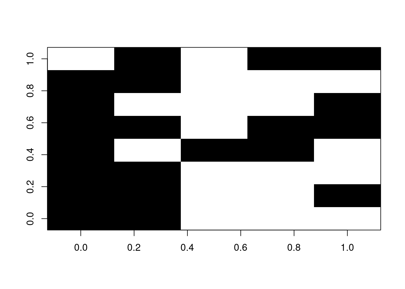
But you can also use this option to only select some specific edges and modify them (for example making them all equal to one):
## Adding a fixed edge length to the green clade
my_tree_modif <- my_tree
green_clade <- which(clade_edges == "darkgreen")
my_tree_modif$edge.length[green_clade] <- 1
plot(ladderize(my_tree_modif), show.tip.label = FALSE,
     edge.color = clade_edges)
6.6 MCMCglmm utilities
Since version 1.7, the dispRity package contains several utility functions for manipulating "MCMCglmm" (that is, objects returned by the function MCMCglmm::MCMCglmm).
These objects are a modification of the mcmc object (from the package coda) and can be sometimes cumbersome to manipulate because of the huge amount of data in it.
You can use the functions MCMCglmm.traits for extracting the number of traits, MCMCglmm.levels for extracting the level names, MCMCglmm.sample for sampling posterior IDs and MCMCglmm.covars for extracting variance-covariance matrices. You can also quickly calculate the variance (or relative variance) for each terms in the model using MCMCglmm.variance (the variance is calculated as the sum of the diagonal of each variance-covariance matrix for each term).
## Loading the charadriiformes data that contains a MCMCglmm object
data(charadriiformes)
my_MCMCglmm <- charadriiformes$posteriors

## Which traits where used in this model?
MCMCglmm.traits(my_MCMCglmm)
## [1] "PC1" "PC2" "PC3"## Which levels where used for the model's random terms and/or residuals?
MCMCglmm.levels(my_MCMCglmm)## random random random random
## "animal:clade_1" "animal:clade_2" "animal:clade_3" "animal"
## residual
## "units"## The level names are converted for clarity but you can get them unconverted
## (i.e. as they appear in the model)
MCMCglmm.levels(my_MCMCglmm, convert = FALSE)## random random
## "us(at.level(clade, 1):trait):animal" "us(at.level(clade, 2):trait):animal"
## random random
## "us(at.level(clade, 3):trait):animal" "us(trait):animal"
## residual
## "us(trait):units"## [1] 749 901## Extracting these two random samples
my_covars <- MCMCglmm.covars(my_MCMCglmm, sample = random_samples)
## Plotting the variance for each term in the model
boxplot(MCMCglmm.variance(my_MCMCglmm), horizontal = TRUE, las = 1,
xlab = "Relative variance",
main = "Variance explained by each term")
See more in the $covar section on what to do with these "MCMCglmm" objects.
6.7 pair.plot
This utility function allows to plot a matrix image of pairwise comparisons. This can be useful when getting pairwise comparisons and if you’d like to see at a glance which pairs of comparisons have high or low values.
## Random data
data <- matrix(data = runif(42), ncol = 2)

## Plotting the first column as a pairwise comparisons
pair.plot(data, what = 1, col = c("orange", "blue"), legend = TRUE,
          diag = 1)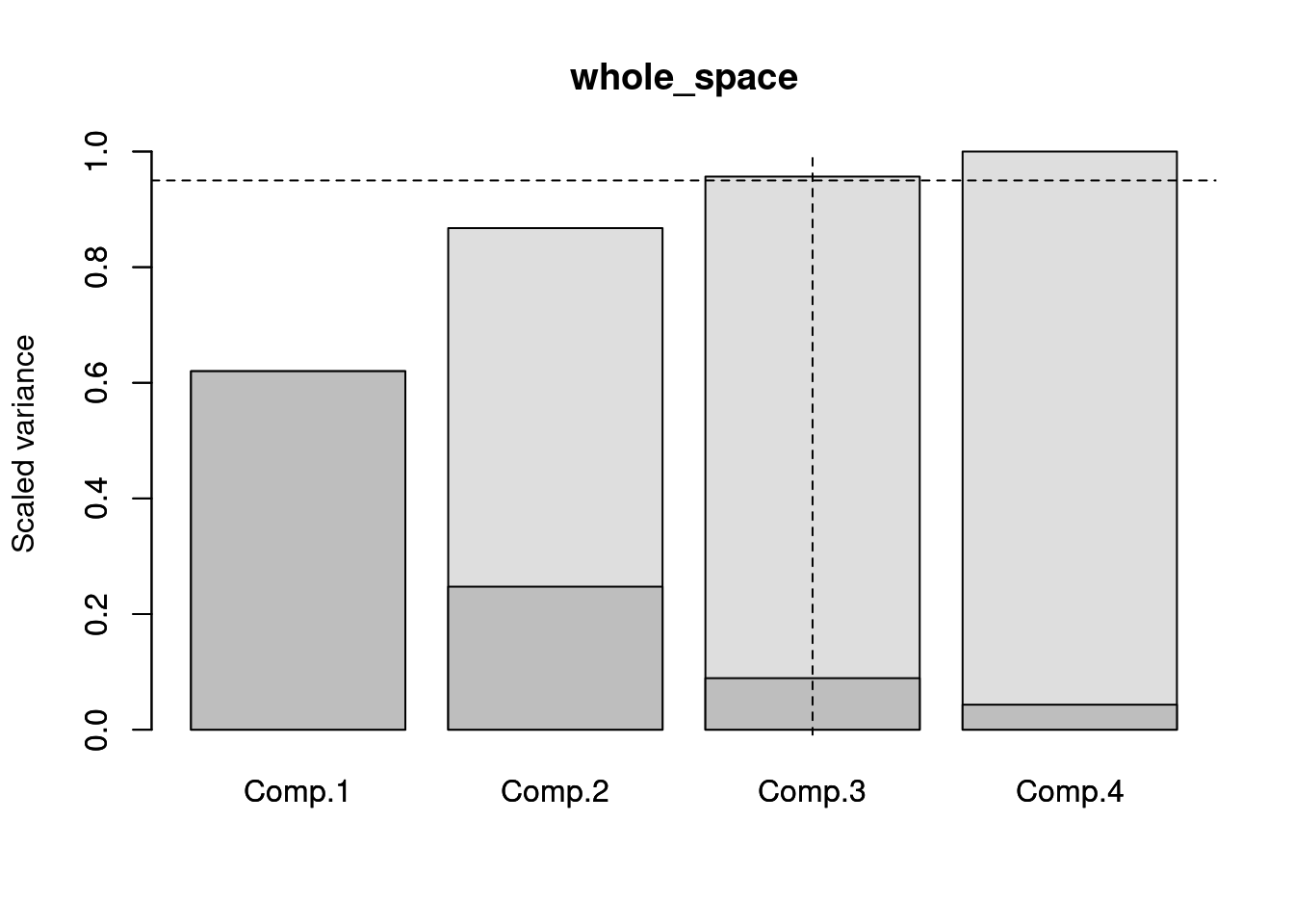
Here blue squares are ones that have a high value and orange ones the ones that have low values.
Note that the values plotted correspond the first column of the data as designated by what = 1.
It is also possible to add some tokens or symbols to quickly highlight to specific cells, for example which elements in the data are below a certain value:
## The same plot as before without the diagonal being
## the maximal observed value
pair.plot(data, what = 1, col = c("orange", "blue"), legend = TRUE,
          diag = "max")
## Highlighting with an asterisk which squares have a value
## below 0.2
pair.plot(data, what = 1, binary = 0.2, add = "*", cex = 2)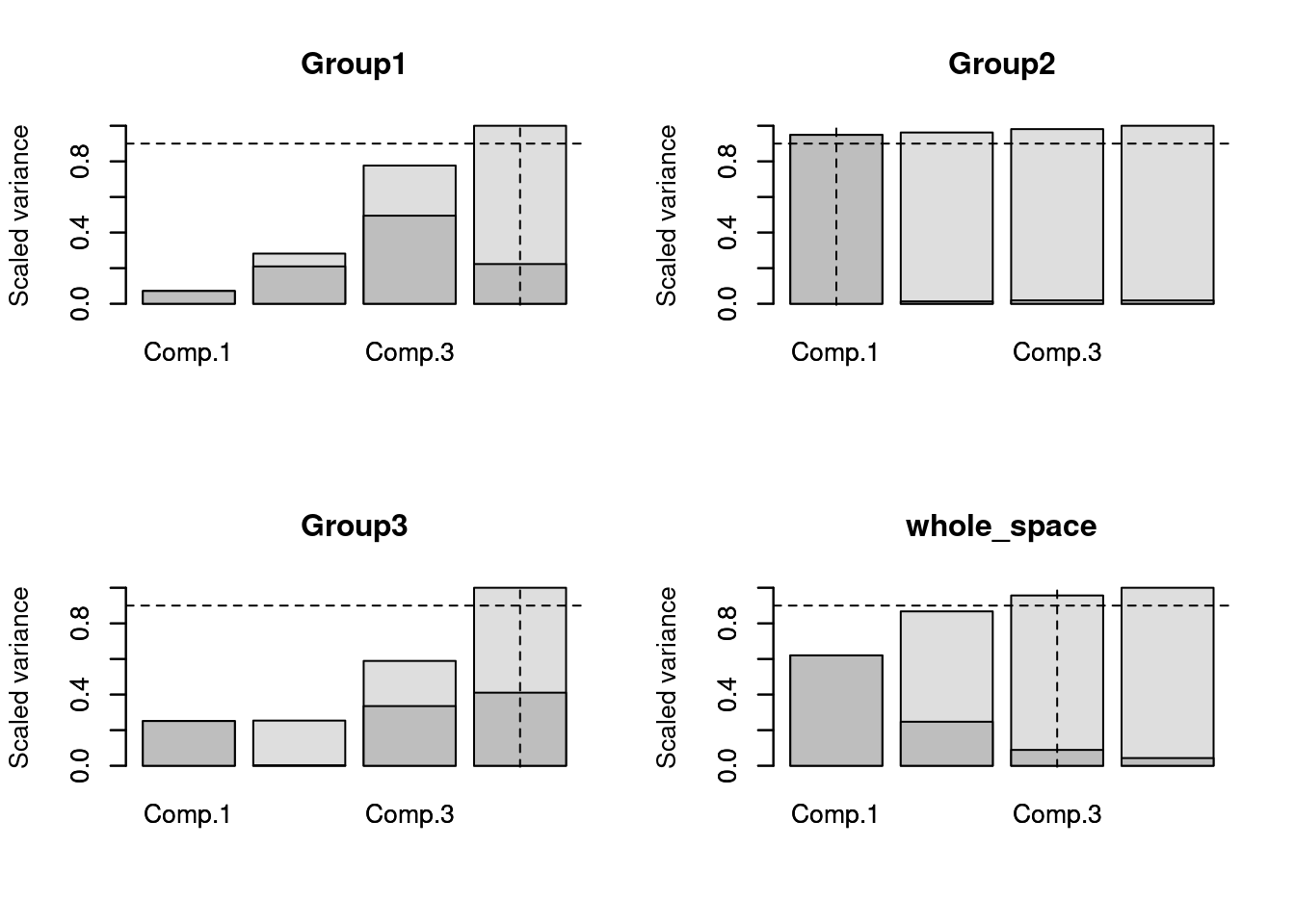
This function can also be used as a binary display when running a series of pairwise t-tests.
For example, the following script runs a wilcoxon test between the time-slices from the disparity example dataset and displays in black which pairs of slices have a p-value below 0.05:
## Loading disparity data
data(disparity)

## Testing the pairwise difference between slices
tests <- test.dispRity(disparity, test = wilcox.test, correction = "bonferroni")

## Plotting the significance
pair.plot(as.data.frame(tests), what = "p.value", binary = 0.05)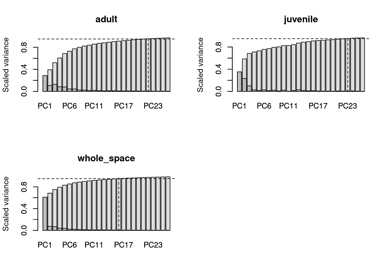
6.8 reduce.matrix
This function allows to reduce columns or rows of a matrix to make sure that there is enough overlap for further analysis.
This is particularly useful if you are going to use distance matrices since it uses the vegan::vegdist function to test whether distances can be calculated or not.
For example, if we have a patchy matrix like so (where the black squares represent available data):
set.seed(1)
## A 10*5 matrix
na_matrix <- matrix(rnorm(50), 10, 5)
## Making sure some rows don't overlap
na_matrix[1, 1:2] <- NA
na_matrix[2, 3:5] <- NA
## Adding 50% NAs
na_matrix[sample(1:50, 25)] <- NA
## Illustrating the gappy matrix
image(t(na_matrix), col = "black")
We can use the reduce.matrix to double check whether any rows cannot be compared.
The functions needs as an input the type of distance that will be used, say a "gower" distance:
## $rows.to.remove
## [1] "9" "1"
##
## $cols.to.remove
## NULL
We can not remove the rows 1 and 9 and see if that improved the overlap:

6.9 select.axes
This function allows you to select which axes (or how many of them) are relevant in your trait space analyses. Usually, when the trait space is an ordination, workers select a certain number of axes to reduce the dimensionality of the dataset by removing axes that contain relatively little information. This is often done by selecting the axes from which the cumulative individual variance is lower than an arbitrary threshold. For example, all the axes that contain together 0.95 of the variance:
## The USArrest example in R
ordination <- princomp(USArrests, cor = TRUE)

## The loading of each variable
loadings(ordination)
##
## Loadings:
## Comp.1 Comp.2 Comp.3 Comp.4
## Murder 0.536 0.418 0.341 0.649
## Assault 0.583 0.188 0.268 -0.743
## UrbanPop 0.278 -0.873 0.378 0.134
## Rape 0.543 -0.167 -0.818
##
## Comp.1 Comp.2 Comp.3 Comp.4
## SS loadings 1.00 1.00 1.00 1.00
## Proportion Var 0.25 0.25 0.25 0.25
## Cumulative Var 0.25 0.50 0.75 1.00## Or the same operation but manually
variances <- apply(ordination$scores, 2, var)
scaled_variances <- variances/sum(variances)
sumed_variances <- cumsum(scaled_variances)
round(rbind(variances, scaled_variances, sumed_variances), 3)## Comp.1 Comp.2 Comp.3 Comp.4
## variances 2.531 1.010 0.364 0.177
## scaled_variances 0.620 0.247 0.089 0.043
## sumed_variances 0.620 0.868 0.957 1.000In this example, you can see that the three first axes are required to have at least 0.95 of the variance.
You can do that automatically in dispRity using the select.axes function.
## The first 3 dimensions are needed to express at least 95% of the variance in the whole trait space.
## You can use x$dimensions to select them or use plot(x) and summary(x) to summarise them.
This function does basically what the script above does and allows the results to be plotted or summarised into a table.
##             Comp.1.var Comp.1.sum Comp.2.var Comp.2.sum Comp.3.var Comp.3.sum
## whole_space       0.62       0.62      0.247      0.868      0.089      0.957
##             Comp.4.var Comp.4.sum
## whole_space      0.043          1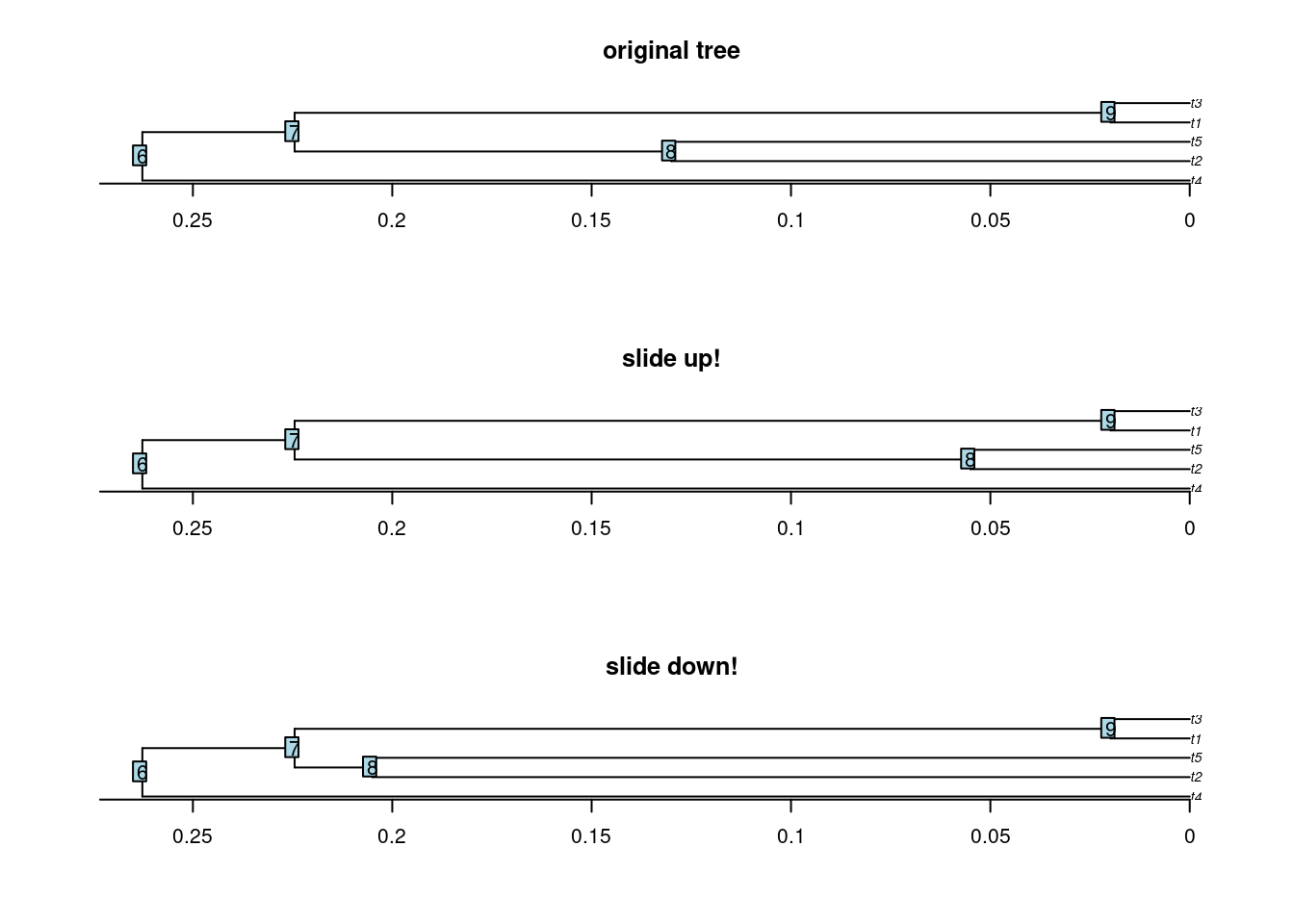
## [1] 1 2 3However, it might be interesting to not only consider the variance within the whole trait space but also among groups of specific interest.
E.g. if the 95% of the variance is concentrated in the two first axes for the whole trait space, that does not automatically mean that it is the case for each subset in this space. Some subset might require more than the two first axes to express 95% of their variance!
You can thus use the select.axes function to look at the results per group as well as through the whole trait space.
Note that you can always change the threshold value (default is 0.95). Here for example we set it to 0.9 (we arbitrarily decide that explain 90% of the variance is enough).
## Creating some groups of stats
states_groups <- list("Group1" = c("Mississippi","North Carolina",
                                   "South Carolina", "Georgia", "Alabama",
                                   "Alaska", "Tennessee", "Louisiana"),
                      "Group2" = c("Florida", "New Mexico", "Michigan",
                                   "Indiana", "Virginia", "Wyoming", "Montana",
                                   "Maine", "Idaho", "New Hampshire", "Iowa"),
                      "Group3" = c("Rhode Island", "New Jersey", "Hawaii", "Massachusetts"))
## Running the same analyses but per groups
selected <- select.axes(ordination, group = states_groups, threshold = 0.9)
## Plotting the results
plot(selected)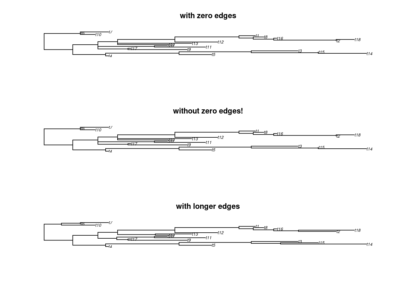
As you can see here, the whole space requires the three first axes to explain at least 90% of the variance (in fact, 95% as seen before).
However, different groups have a different story!
The Group 1 and 3 requires 4 dimensions whereas Group 2 requires only 1 dimensions (note how for Group 3, there is actually nearly no variance explained on the second axes)!
Using this method, you can safely use the four axes returned by the function (selected$dimensions) so that every group has at least 90% of their variance explained in the trait space.
If you’ve used the function if you’ve already done some grouping in your disparity analyses (e.g. using the function custom.subsets or chrono.subsets), you can use the generated dispRity to automatise this analyses:
## Loading the dispRity package demo data
data(demo_data)
## A dispRity object with two groups
demo_data$hopkins
## ---- dispRity object ----
## 2 customised subsets for 46 elements in one matrix:
## adult, juvenile.
## $adult
##  [1]  1  2  3  4  5  6  7  8  9 10 11 12 13 14 15 16 17 18 19 20 21 22
##
## $juvenile
##  [1]  1  2  3  4  5  6  7  8  9 10 11 12 13 14 15 16 17 18 19 20 21 22 23
##
## $whole_space
## [1] 1 2 3 4 5 6 7 8 9 10 11 12 13 14 15 166.10 set.root.time
This function can be used to easily add a $root.time element to "phylo" or "multiPhylo" objects.
This $root.time element is used by dispRity and several packages (e.g. Claddis and paleotree) to scale the branch length units of a tree allowing them to be usually expressed in million of years (Mya).
For example, on a standard random tree, no $root.time exist so the edge lengths are not expressed in any specific unit:
## NULLYou can add a root time by either manually setting it:
## Adding an arbitrary root time
my_tree_arbitrary <- my_tree
## Setting the age of the root to 42
my_tree_arbitrary$root.time <- 42
Or by calculating it automatically from the cumulated branch length information (making the youngest tip age 0 and the oldest the total age/depth of the tree)
## Calculating the root time from the present
my_tree_aged <- my_tree
my_tree_aged <- set.root.time(my_tree)
If you want the youngest tip to not be of age 0, you can define an arbitrary age for it and recalculate the age of the root from there using the present argument (say the youngest tip is 42 Mya old):
This function also works with a distribution of trees ("multiPhylo").
6.11 slice.tree
This function is a modification of the paleotree::timeSliceTree function that allows to make slices through a phylogenetic tree.
Compared to the paleotree::timeSliceTree, this function allows a model to decide which tip or node to use when slicing through a branch (whereas paleotree::timeSliceTree always choose the first available tip alphabetically).
The models for choosing which tip or node are the same as the ones used in the chrono.subsets and are described in chapter 03: specific tutorials.
The function works by using at least a tree, a slice age and a model:
set.seed(1)
## Generate a random ultrametric tree
tree <- rcoal(20)
## Add some node labels
tree$node.label <- letters[1:19]
## Add its root time
tree$root.time <- max(tree.age(tree)$ages)

## Slicing the tree at age 0.75
tree_75 <- slice.tree(tree, age = 0.75, "acctran")

## Showing both trees
par(mfrow = c(1,2))
plot(tree, main = "original tree")
axisPhylo() ; nodelabels(tree$node.label, cex = 0.8)
abline(v = (max(tree.age(tree)$ages) - 0.75), col = "red")
plot(tree_75, main = "sliced tree")
6.12 slide.nodes and remove.zero.brlen
This function allows to slide nodes along a tree! In other words it allows to change the branch length leading to a node without modifying the overall tree shape. This can be useful to add some value to 0 branch lengths for example.
The function works by taking a node (or a list of nodes), a tree and a sliding value. The node will be moved “up” (towards the tips) for the given sliding value. You can move the node “down” (towards the roots) using a negative value.
set.seed(42)
## Generating simple coalescent tree
tree <- rcoal(5)

## Sliding node 8 up and down
tree_slide_up <- slide.nodes(8, tree, slide = 0.075)
tree_slide_down <- slide.nodes(8, tree, slide = -0.075)

## Display the results
par(mfrow = c(3,1))
plot(tree, main = "original tree") ; axisPhylo() ; nodelabels()
plot(tree_slide_up, main = "slide up!") ; axisPhylo() ; nodelabels()
plot(tree_slide_down, main = "slide down!") ; axisPhylo() ; nodelabels()
The remove.zero.brlen is a “clever” wrapping function that uses the slide.nodes function to stochastically remove zero branch lengths across a whole tree.
This function will slide nodes up or down in successive postorder traversals (i.e. going down the tree clade by clade) in order to minimise the number of nodes to slide while making sure there are no silly negative branch lengths produced!
By default it is trying to slide the nodes using 1% of the minimum branch length to avoid changing the topology too much.
set.seed(42)
## Generating a tree
tree <- rtree(20)

## Adding some zero branch lengths (5)
tree$edge.length[sample(1:Nedge(tree), 5)] <- 0

## And now removing these zero branch lengths!
tree_no_zero <- remove.zero.brlen(tree)

## Exaggerating the removal (to make it visible)
tree_exaggerated <- remove.zero.brlen(tree, slide = 1)

## Check the differences
any(tree$edge.length == 0)
## [1] TRUE## [1] FALSE## [1] FALSE## Display the results
par(mfrow = c(3,1))
plot(tree, main = "with zero edges")
plot(tree_no_zero, main = "without zero edges!")
plot(tree_exaggerated, main = "with longer edges")
6.13 tree.age
This function allows to quickly calculate the ages of each tips and nodes present in a tree.
##      ages elements
## 1  0.7068       t7
## 2  0.1417       t2
## 3  0.0000       t3
## 4  1.4675       t8
## 5  1.3656       t1
## 6  1.8949       t5
## 7  1.5360       t6
## 8  1.4558       t9
## 9  0.8147      t10
## 10 2.3426       t4
## 11 3.0111       11
## 12 2.6310       12
## 13 1.8536       13
## 14 0.9189       14
## 15 0.2672       15
## 16 2.6177       16
## 17 2.2353       17
## 18 2.1356       18
## 19 1.6420       19
It also allows to set the age of the root of the tree:
##        ages elements
## 1   23.4717       t7
## 2    4.7048       t2
## 3    0.0000       t3
## 4   48.7362       t8
## 5   45.3517       t1
## 6   62.9315       t5
## 7   51.0119       t6
## 8   48.3486       t9
## 9   27.0554      t10
## 10  77.7998       t4
## 11 100.0000       11
## 12  87.3788       12
## 13  61.5593       13
## 14  30.5171       14
## 15   8.8746       15
## 16  86.9341       16
## 17  74.2347       17
## 18  70.9239       18
## 19  54.5330       19
Usually tree age is calculated from the present to the past (e.g. in million years ago) but it is possible to reverse it using the order = present option:
##      ages elements
## 1  2.3043       t7
## 2  2.8694       t2
## 3  3.0111       t3
## 4  1.5436       t8
## 5  1.6455       t1
## 6  1.1162       t5
## 7  1.4751       t6
## 8  1.5553       t9
## 9  2.1964      t10
## 10 0.6685       t4
## 11 0.0000       11
## 12 0.3800       12
## 13 1.1575       13
## 14 2.0922       14
## 15 2.7439       15
## 16 0.3934       16
## 17 0.7758       17
## 18 0.8755       18
## 19 1.3690       19
6.14 multi.ace
This function allows to run ancestral characters estimations on multiple trees.
In it’s most basic structure (e.g. using all default arguments) this function is using a mix of ape::ace and castor::asr_mk_model depending on the data and the situation and is generally faster than both functions when applied to a list of trees.
However, this function provides also some more complex and modular functionalities, especially appropriate when using discrete morphological character data.
6.14.1 Using different character tokens in different situations
This data can be often coded in non-standard way with different character tokens having different meanings.
For example, in some datasets the token - can mean “the trait is inapplicable” but this can be also coded by the more conventional NA or can mean “this trait is missing” (often coded ?).
This makes the meaning of specific tokens idiosyncratic to different matrices.
For example we can have the following discrete morphological matrix with all the data encoded:
set.seed(42)
## A random tree with 10 tips
tree <- rcoal(10)
## Setting up the parameters
my_rates = c(rgamma, rate = 10, shape = 5)

## Generating a bunch of trees
multiple_trees <- rmtree(5, 10)

## A random Mk matrix (10*50)
matrix_simple <- sim.morpho(tree, characters = 50, model = "ER", rates = my_rates,
                            invariant = FALSE)
matrix_simple[1:10, 1:10]
## [,1] [,2] [,3] [,4] [,5] [,6] [,7] [,8] [,9] [,10]
## t8 "1" "1" "1" "1" "0" "0" "0" "0" "0" "1"
## t3 "1" "1" "1" "1" "0" "0" "0" "0" "0" "1"
## t2 "1" "1" "1" "1" "0" "1" "1" "1" "0" "1"
## t1 "1" "1" "1" "1" "0" "0" "1" "1" "0" "1"
## t10 "1" "1" "1" "1" "0" "0" "1" "0" "1" "1"
## t9 "1" "1" "1" "1" "0" "0" "1" "0" "0" "1"
## t5 "0" "0" "0" "0" "1" "1" "1" "0" "0" "0"
## t6 "0" "0" "0" "0" "1" "1" "1" "0" "0" "0"
## t4 "0" "0" "0" "0" "1" "0" "0" "0" "1" "0"
## t7 "0" "0" "0" "0" "1" "0" "0" "0" "1" "0"But of course, as mentioned above, in practice, such matrices have more nuance and can including missing characters, ambiguous characters, multi-state characters, inapplicable characters, etc… All these coded and defined by different authors using different tokens (or symbols). Let’s give it a go and transform this simple data to something more messy:
## Modify the matrix to contain missing and special data
matrix_complex <- matrix_simple
## Adding 50 random "-" tokens
matrix_complex[sample(1:length(matrix_complex), 50)] <- "-"
## Adding 50 random "?" tokens
matrix_complex[sample(1:length(matrix_complex), 50)] <- "?"
## Adding 50 random "0%2" tokens
matrix_complex[sample(1:length(matrix_complex), 50)] <- "0%2"
matrix_complex[1:10,1:10]
## [,1] [,2] [,3] [,4] [,5] [,6] [,7] [,8] [,9] [,10]
## t8 "1" "1" "1" "1" "?" "0" "0" "0" "0" "0%2"
## t3 "1" "-" "1" "1" "?" "0" "0" "0" "0" "1"
## t2 "1" "1" "1" "0%2" "0" "0%2" "1" "1" "0" "1"
## t1 "1" "1" "1" "1" "0" "0" "1" "?" "0" "1"
## t10 "1" "0%2" "1" "1" "-" "?" "0%2" "0%2" "1" "1"
## t9 "1" "1" "?" "1" "0%2" "0" "1" "0" "0" "1"
## t5 "0" "-" "?" "0" "1" "1" "1" "0" "0" "-"
## t6 "0" "-" "0" "0" "1" "1" "-" "-" "?" "0"
## t4 "?" "0" "0" "0" "1" "0" "0" "0" "1" "0"
## t7 "0" "0" "0" "0%2" "1" "0" "0" "-" "1" "-"In multi.ace you can specify what all these tokens actually mean and how the code should interpret them.
For example, - often means inapplicable data (i.e. the specimen does not have the coded feature, for example, the colour of the tail of a tailless bird); or ? that often means missing data (i.e. it is unknown if the specimen has a tail or not since only the head was available).
And more than the differences in meaning between these characters, different people treat these characters differently even if they have the same meaning for the token.
For example, one might want to treat - as meaning “we don’t know” (which will be treated by the algorithm as “any possible trait value”) or “we know, and it’s no possible” (which will be treated by the algorithm as NA).
Because of this situation, multi.ace allows combining any special case marked with a special token to a special behaviour.
For example we might want to create a special case called "missing" (i.e. the data is missing) that we want to denote using the token "?" and we can specify the algorithm to treat this "missing" cases ("?") as treating the character token value as “any possible values”.
This behaviour can be hard coded by providing a function with the name of the behaviour.
For example:
## The specific token for the missing cases (note the "\\" for protecting the value)
special.tokens <- c("missing" = "\\?")

## The behaviour for the missing cases (?)
special.behaviour <- list(missing <- function(x, y) return(y))
## Where x is the input value (here "?") and y is all the possible normal values for the character
This example shows a very common case (and is actually used by default, more on that below) but this architecture allows for very modular combination of tokens and behaviours.
For example, in our code above we introduced the token "%" which is very odd (to my knowledge) and might mean something very specific in our case.
Say we want to call this case "weirdtoken" and mean that whenever this token is encountered in a character, it should be interpreted by the algorithm as the values 1 and 2, no matter what:
## Set a list of extra special tokens
my_spec_tokens <- c("weirdtoken" = "\\%")

## Weird tokens are considered as state 0 and 3
my_spec_behaviours <- list()
my_spec_behaviours$weirdtoken <- function(x,y) return(c(1,2))
If you don’t need/don’t have any of this specific tokens, don’t worry, most special but common tokens are handled by default as such:
## The token for missing values:
default_tokens <- c("missing"      = "\\?",
## The token for inapplicable values:
                    "inapplicable" = "\\-",
## The token for polymorphisms:
                    "polymorphism" = "\\&",
## The token for uncertainties:
                    "uncertanity"  = "\\/")
With the following associated default behaviours
## Treating missing data as all data values
default_behaviour <- list(missing      <- function(x,y) y,
## Treating inapplicable data as all data values (like missing)
                          inapplicable <- function(x, y) y,
## Treating polymorphisms as all values present:
                          polymorphism <- function(x,y) strsplit(x, split = "\\&")[[1]],
## Treating uncertainties as all values present (like polymorphisms):
                          uncertanity  <- function(x,y) strsplit(x, split = "\\/")[[1]])
We can then use these token description along with our complex matrix and our list of trees to run the ancestral states estimations as follows:
## Running ancestral states
ancestral_states <- multi.ace(matrix_complex, multiple_trees,
                              special.tokens = my_spec_tokens,
                              special.behaviours = my_spec_behaviours,
                              verbose = TRUE)
## Preparing the data:...## Warning: The character 39 is invariant (using the current special behaviours
## for special characters) and is simply duplicated for each node.## ..Done.
## Running ancestral states estimations:.....................................................................................................................................................................................................................................................Done.## This outputs a list of ancestral parts of the matrices for each tree
## For example, here's the first one:
ancestral_states[[1]][1:9, 1:10]## [,1] [,2] [,3] [,4] [,5] [,6] [,7] [,8] [,9] [,10]
## n1 "1" "1" "1" "1" "1" "0/1/2" "1" "0" "0" "1"
## n2 "1" "1" "1" "1" "0/1" "0/1/2" "0/1" "0" "0" "1"
## n3 "1" "1" "1" "1" "0/1" "0/1/2" "0" "0" "0" "1"
## n4 "1" "1" "1" "1" "0" "0/1/2" "1" "1" "0" "1"
## n5 "1" "1" "1" "1" "1" "0/1/2" "1" "0" "0" "1"
## n6 "1" "1" "1" "1" "1" "0/1/2" "1" "0" "0" "1"
## n7 "0" "0/1" "0/1" "0" "1" "1" "1" "0" "0" "0/1"
## n8 "0" "0" "0" "0" "1" "0/1/2" "0" "0" "1" "0"
## n9 "0" "0" "0" "0" "1" "1" "0" "0" "1" "0"Note that there are many different options that are not covered here.
For example, you can use different models for each character via the models argument, you can specify how to handle uncertainties via the threshold argument, use a branch length modifier (brlen.multiplier), specify the type of output, etc…
6.14.2 Feeding the results to char.diff to get distance matrices
After running your ancestral states estimations, it is not uncommon to then use these resulting data to calculate the distances between taxa and then ordinate the results to measure disparity.
You can do that using the char.diff function described above but instead of measuring the distances between characters (columns) you can measure the distances between species (rows).
You might notice that this function uses the same modular token and behaviour descriptions.
That makes sense because they’re using the same core C functions implemented in dispRity that greatly speed up distance calculations.
## Running ancestral states
## and outputing a list of combined matrices (tips and nodes)
ancestral_states <- multi.ace(matrix_complex, multiple_trees,
                              special.tokens = my_spec_tokens,
                              special.behaviours = my_spec_behaviours,
                              output = "combined.matrix",
                              verbose = TRUE)
## Preparing the data:...## Warning: The character 39 is invariant (using the current special behaviours
## for special characters) and is simply duplicated for each node.## ..Done.
## Running ancestral states estimations:.....................................................................................................................................................................................................................................................Done.We can then feed these matrices directly to char.diff, say for calculating the “MORD” distance:
## Measuring the distances between rows using the MORD distance
distances <- lapply(ancestral_states, char.diff, method = "mord", by.col = FALSE)
And we now have a list of distances matrices with ancestral states estimated!
6.14.3 Running ancestral states estimations for continuous characters
You can also run multi.ace on continuous characters.
The function detects any continuous characters as being of class "numeric" and runs them using the ape::ace function.
set.seed(1)
## Creating three coalescent trees
my_trees <- replicate(3, rcoal(15), simplify = FALSE)
## Adding node labels
my_trees <- lapply(my_trees, makeNodeLabel)
## Making into a multiPhylo object
class(my_trees) <- "multiPhylo"

## Creating a matrix of continuous characters
data <- space.maker(elements = 15, dimensions = 5, distribution = rnorm,
                    elements.name = my_trees[[1]]$tip.label)
With such data and trees you can easily run the multi.ace estimations.
By default, the estimations use the default arguments from ape::ace, knowingly a Brownian Motion (model = "BM") with the REML method (method = "REML"; this method “first estimates the ancestral value at the root (aka, the phylogenetic mean), then the variance of the Brownian motion process is estimated by optimizing the residual log-likelihood” - from ?ape::ace).
## Warning in sqrt(1/out$hessian): NaNs produced
## Warning in sqrt(1/out$hessian): NaNs produced
## Warning in sqrt(1/out$hessian): NaNs produced
## Warning in sqrt(1/out$hessian): NaNs produced
## Warning in sqrt(1/out$hessian): NaNs produced
## Warning in sqrt(1/out$hessian): NaNs produced
## Warning in sqrt(1/out$hessian): NaNs produced
## Warning in sqrt(1/out$hessian): NaNs produced
## Warning in sqrt(1/out$hessian): NaNs produced
## Warning in sqrt(1/out$hessian): NaNs produced
## Warning in sqrt(1/out$hessian): NaNs produced
## Warning in sqrt(1/out$hessian): NaNs produced
## Warning in sqrt(1/out$hessian): NaNs produced
## List of 3
## $ : num [1:14, 1:5] -0.191 -0.155 -0.227 -0.17 0.138 ...
## ..- attr(*, "dimnames")=List of 2
## .. ..$ : chr [1:14] "Node1" "Node2" "Node3" "Node4" ...
## .. ..$ : NULL
## $ : num [1:14, 1:5] -0.385 -0.552 -0.445 -0.435 -0.478 ...
## ..- attr(*, "dimnames")=List of 2
## .. ..$ : chr [1:14] "Node1" "Node2" "Node3" "Node4" ...
## .. ..$ : NULL
## $ : num [1:14, 1:5] -0.3866 -0.2232 -0.0592 -0.7246 -0.2253 ...
## ..- attr(*, "dimnames")=List of 2
## .. ..$ : chr [1:14] "Node1" "Node2" "Node3" "Node4" ...
## .. ..$ : NULLThis results in three matrices with ancestral states for the nodes.
When using continuous characters, however, you can output the results directly as a dispRity object that allows visualisation and other normal dispRity pipeline:
## Running multi.ace on continuous data
my_ancestral_states <- multi.ace(data, my_trees, output = "dispRity")
## Warning in sqrt(1/out$hessian): NaNs produced
## Warning in sqrt(1/out$hessian): NaNs produced
## Warning in sqrt(1/out$hessian): NaNs produced
## Warning in sqrt(1/out$hessian): NaNs produced
## Warning in sqrt(1/out$hessian): NaNs produced
## Warning in sqrt(1/out$hessian): NaNs produced
## Warning in sqrt(1/out$hessian): NaNs produced
## Warning in sqrt(1/out$hessian): NaNs produced
## Warning in sqrt(1/out$hessian): NaNs produced
## Warning in sqrt(1/out$hessian): NaNs produced
## Warning in sqrt(1/out$hessian): NaNs produced
## Warning in sqrt(1/out$hessian): NaNs produced
## Warning in sqrt(1/out$hessian): NaNs produced
You can also mix continuous and discrete characters together.
By default the multi.ace detects which character is of which type and applies the correct estimations based on that.
However you can always specify models or other details character per characters.
## Adding two discrete characters
data <- as.data.frame(data)
data <- cbind(data, "new_char" = as.character(sample(1:2, 15, replace = TRUE)))
data <- cbind(data, "new_char2" = as.character(sample(1:2, 15, replace = TRUE)))

## Setting up different models for each characters
## BM for all 5 continuous characters
## and ER and ARD for the two discrete ones
my_models <- c(rep("BM", 5), "ER", "ARD")

## Running the estimation with the specified models
my_ancestral_states <- multi.ace(data, my_trees, models = my_models)
## Warning in sqrt(1/out$hessian): NaNs produced
## Warning in sqrt(1/out$hessian): NaNs produced
## Warning in sqrt(1/out$hessian): NaNs produced
## Warning in sqrt(1/out$hessian): NaNs produced
## Warning in sqrt(1/out$hessian): NaNs produced
## Warning in sqrt(1/out$hessian): NaNs produced
## Warning in sqrt(1/out$hessian): NaNs produced
## Warning in sqrt(1/out$hessian): NaNs produced
## Warning in sqrt(1/out$hessian): NaNs produced
## Warning in sqrt(1/out$hessian): NaNs produced
## Warning in sqrt(1/out$hessian): NaNs produced
## Warning in sqrt(1/out$hessian): NaNs produced
## Warning in sqrt(1/out$hessian): NaNs producedOf course all the options discussed in the first part above also can apply here!