Stat 545 getting data from the Web
Andrew MacDonald
2015-11-24
library(dplyr)
library(knitr)
# library(devtools)
Introduction
All this and more is described at the rOpenSci repository of R tools for interacting with the internet
There are many ways to obtain data from the Internet; let’s consider four categories:
- click-and-download on the internet as a “flat” file, such as .csv, .xls
- install-and-play an API for which someone has written a handy R package
- API-query published with an unwrapped API
- Scraping implicit in an html website
Click-and-Download
In the simplest case, the data you need is already on the internet in a tabular format. There are a couple of strategies here:
use
read.csvorreadr::read_csvto read the data straight into R.use the command line program
curlto do that work, and place it in a Makefile or shell script (see the Make lesson for how to do that).
The second case is most useful when the data you want has been provided in a format that needs cleanup. For example, the World Value Survey makes several datasets available as Excel sheets. The safest option here is to download the .xls file, then read it into R with readxl::read_excel() or something similar. An exception to this is data provided as Google Spreadsheets, which can be read straight into R using the googlesheets package.
from ropensci web services page:
downloader::download()for SSLcurl::curl()for SSL.httr::GETdata read this way needs to be parsed later with read.tablerio::import()can “read a number of common data formats directly from an https:// URL”. Isn’t that very similar to the previous?
What about packages that install data?
Data supplied on the web
Many times, the data that you want is not already organized into one or a few tables that you can read directly into R. More frequently, you find this data is given in the form of an API. Application Programming Interfaces (APIs) are descriptions of the kind of requests that can be made of a certain piece of software, and descriptions of the kind of answers that are returned. Many sources of data – databases, websites, services – have made all (or part) of their data available via APIs over the internet. Computer programs (“clients”) can make requests of the server, and the server will respond by sending data (or an error message). This client can be many kinds of other programs or websites, including R running from your laptop.
install-and-play
Many common web services and APIs have been “wrapped”, i.e. R functions have been written around them which send your query to the server and format the response.
Why do we want this?
- provenance
- reproducible
- updating
- ease
- scaling
Sightings of birds: rebird
rebird is an R interface for the ebird database. e-Bird lets birders upload sightings of birds, and allows everyone access to those data.
rebird is on CRAN.
install.packages("rebird")library(rebird)Search birds by geography
the ebird website categorizes some popular locations as “Hotspots”. These are areas where there are both lots of birds and lots of birders. Once such location is at Iona Island, near Vancouver. You can see data for this site at http://ebird.org/ebird/hotspot/L261851
At that link, you can see a page like this:
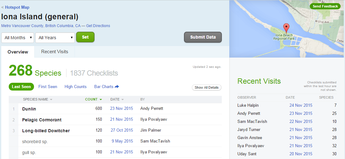
The data already look to be organized in a data frame! rebird allows us to read these data directly into R. (The ID code for Iona Island is **“L261851**)
ebirdhotspot(locID = "L261851") %>%
  head() %>%
  kable()
## Warning: `rbind_all()` is deprecated. Please use `bind_rows()` instead.| obsDt | lng | locName | obsValid | comName | obsReviewed | sciName | locationPrivate | howMany | lat | locID |
|---|---|---|---|---|---|---|---|---|---|---|
| 2015-11-24 11:41 | -123.2111 | Iona Island (general) | TRUE | Snow Goose | FALSE | Chen caerulescens | FALSE | 40 | 49.22133 | L261851 |
| 2015-11-24 11:41 | -123.2111 | Iona Island (general) | TRUE | Gadwall | FALSE | Anas strepera | FALSE | 10 | 49.22133 | L261851 |
| 2015-11-24 11:41 | -123.2111 | Iona Island (general) | TRUE | American Wigeon | FALSE | Anas americana | FALSE | 25 | 49.22133 | L261851 |
| 2015-11-24 11:41 | -123.2111 | Iona Island (general) | TRUE | Mallard | FALSE | Anas platyrhynchos | FALSE | NA | 49.22133 | L261851 |
| 2015-11-24 11:41 | -123.2111 | Iona Island (general) | TRUE | Northern Pintail | FALSE | Anas acuta | FALSE | 35 | 49.22133 | L261851 |
| 2015-11-24 11:41 | -123.2111 | Iona Island (general) | TRUE | Green-winged Teal | FALSE | Anas crecca | FALSE | 80 | 49.22133 | L261851 |
We can use the function ebirdgeo to get a list for an area. (Note that South and West are negative):
vanbirds <- ebirdgeo(lat = 49.2500, lng = -123.1000)## Warning: `rbind_all()` is deprecated. Please use `bind_rows()` instead.vanbirds %>%
head %>%
kable| obsDt | lng | locName | obsValid | comName | obsReviewed | sciName | locationPrivate | howMany | lat | locID |
|---|---|---|---|---|---|---|---|---|---|---|
| 2015-11-25 15:30 | -123.1754 | Sea Island–Ferguson Rd | TRUE | Song Sparrow | FALSE | Melospiza melodia | FALSE | 1 | 49.20665 | L363627 |
| 2015-11-25 15:30 | -123.1754 | Sea Island–Ferguson Rd | TRUE | European Starling | FALSE | Sturnus vulgaris | FALSE | 5 | 49.20665 | L363627 |
| 2015-11-25 15:30 | -123.1754 | Sea Island–Ferguson Rd | TRUE | Northwestern Crow | FALSE | Corvus caurinus | FALSE | 2 | 49.20665 | L363627 |
| 2015-11-25 15:30 | -123.1754 | Sea Island–Ferguson Rd | TRUE | Short-eared Owl | FALSE | Asio flammeus | FALSE | 2 | 49.20665 | L363627 |
| 2015-11-25 15:30 | -123.1754 | Sea Island–Ferguson Rd | TRUE | Northern Harrier | FALSE | Circus cyaneus | FALSE | 1 | 49.20665 | L363627 |
| 2015-11-25 15:30 | -123.1754 | Sea Island–Ferguson Rd | TRUE | Spotted Towhee | FALSE | Pipilo maculatus | FALSE | 2 | 49.20665 | L363627 |
| Note: Check the | defaults on | this function. e.g. radiu | s of circle | , time of year. |
We can also search by “region”, which refers to short codes which serve as common shorthands for different political units. For example, France is represented by the letters FR
frenchbirds <- ebirdregion("FR")

frenchbirds %>%
  head() %>%
  kable()
Find out WHEN a bird has been seen in a certain place! Choosing a name from vanbirds above (the Bald Eagle):
eagle <- ebirdgeo(species = 'Haliaeetus leucocephalus', lat = 42, lng = -76)

eagle %>%
  head() %>%
  kable()
rebird knows where you are:
ebirdgeo(species = 'Buteo lagopus')Searching geographic info: geonames
# install.packages(geonames)
library(geonames)
There are two things we need to do to be able to use this package to access the geonames API
- go to the geonames site and register an account.
- click here to enable the free web service
- Tell R your geonames username. You could run the line
in R. However this is insecure. We don't want to risk committing this line and pushing it to our public github page! Instead, you should create a file in the same place as your `.Rproj` file. Name this file `.Rprofile`, and add
To that file. Important: Make sure your .Rprofile ends with a blank line!
using Geonames
What can we do? get access to lots of geographical information via the various “web services” see here
countryInfo <- GNcountryInfo()countryInfo %>%
head %>%
kable| continent | capital | languages | geonameId | south | isoAlpha3 | north | fipsCode | population | east | isoNumeric | areaInSqKm | countryCode | west | countryName | continentName | currencyCode |
|---|---|---|---|---|---|---|---|---|---|---|---|---|---|---|---|---|
| EU | Andorra la Vella | ca | 3041565 | 42.4284925987684 | AND | 42.6560438963 | AN | 84000 | 1.78654277783198 | 020 | 468.0 | AD | 1.40718671411128 | Principality of Andorra | Europe | EUR |
| AS | Abu Dhabi | ar-AE,fa,en,hi,ur | 290557 | 22.6333293914795 | ARE | 26.0841598510742 | AE | 4975593 | 56.3816604614258 | 784 | 82880.0 | AE | 51.5833282470703 | United Arab Emirates | Asia | AED |
| AS | Kabul | fa-AF,ps,uz-AF,tk | 1149361 | 29.377472 | AFG | 38.483418 | AF | 29121286 | 74.879448 | 004 | 647500.0 | AF | 60.478443 | Islamic Republic of Afghanistan | Asia | AFN |
| NA | Saint John’s | en-AG | 3576396 | 16.996979 | ATG | 17.729387 | AC | 86754 | -61.672421 | 028 | 443.0 | AG | -61.906425 | Antigua and Barbuda | North America | XCD |
| NA | The Valley | en-AI | 3573511 | 18.166815 | AIA | 18.283424 | AV | 13254 | -62.971359 | 660 | 102.0 | AI | -63.172901 | Anguilla | North America | XCD |
| EU | Tirana | sq,el | 783754 | 39.648361 | ALB | 42.665611 | AL | 2986952 | 21.068472 | 008 | 28748.0 | AL | 19.293972 | Republic of Albania | Europe | ALL |
This country info dataset is very helpful for accessing the rest of the data, because it gives us the standardized codes for country and language.
remixing geonames and rebird:
What are the cities of France?
francedata <- countryInfo %>%
    filter(countryName == "France")
frenchcities <- with(francedata,
GNcities(north = north, east = east, south = south,
west = west, maxRows = 500))
frenchcities %>%
head %>%
kable| lng | geonameId | countrycode | name | fclName | toponymName | fcodeName | wikipedia | lat | fcl | population | fcode |
|---|---|---|---|---|---|---|---|---|---|---|---|
| 2.3488 | 2988507 | FR | Paris | city, village,… | Paris | capital of a political entity | en.wikipedia.org/wiki/Paris | 48.85341 | P | 2138551 | PPLC |
| 4.34878349304199 | 2800866 | BE | Brussels | city, village,… | Brussels | capital of a political entity | en.wikipedia.org/wiki/City_of_Brussels | 50.8504450552593 | P | 1019022 | PPLC |
| 7.44744300842285 | 2661552 | CH | Bern | city, village,… | Bern | capital of a political entity | en.wikipedia.org/wiki/Bern | 46.9480943365053 | P | 121631 | PPLC |
| 6.13 | 2960316 | LU | Luxembourg | city, village,… | Luxembourg | capital of a political entity | en.wikipedia.org/wiki/Luxembourg_%28city%29 | 49.6116667 | P | 76684 | PPLC |
| 7.4166667 | 2993458 | MC | Monaco | city, village,… | Monaco | capital of a political entity | en.wikipedia.org/wiki/Monaco | 43.7333333 | P | 32965 | PPLC |
| -2.10491180419922 | 3042091 | JE | Saint Helier | city, village,… | Saint Helier | capital of a political entity | en.wikipedia.org/wiki/Saint_Helier | 49.1880427659223 | P | 28000 | PPLC |
Wikipedia searching
We can use geonames to search for georeferenced Wikipedia articles. Here are those within 20 Km of Rio de Janerio, comparing results for English-language Wikipedia (lang = "en") and Portuguese-language Wikipedia (lang = "pt"):
rio_english <- GNfindNearbyWikipedia(lat = -22.9083, lng = -43.1964,
                                                                         radius = 20, lang = "en", maxRows = 500)
rio_portuguese <- GNfindNearbyWikipedia(lat = -22.9083, lng = -43.1964,
radius = 20, lang = "pt", maxRows = 500)nrow(rio_english)## [1] 305nrow(rio_portuguese)## [1] 349Searching the Public Library of Science: rplos
PLOS ONE is an open-access journal. They allow access to an impressive range of search tools, and allow you to obtain the full text of their articles.
install.packages("rplos")
## Do this only once:library(rplos)## Loading required package: ggplot2Immediately we get a message. It’s a link to the tutorial on the Ropensci website!. How nice :)
- We also get instructions to create a PLOS account
- Then go to Article Level Metrics http://alm.plos.org/
- click on your name to find your key.
Sys.setenv(PlosApiKey = "Paste your Key in here!!")
key <-  Sys.getenv("PlosApiKey")
alternate strategy for keeping keys: .Rprofile
Remember to protect your key! it is important for your privacy. You know, like a key * Now we follow the ROpenSci tutorial on API keys * Add .Rprofile to your .gitignore !! * Make a .Rprofile file windows tips mac tips * Write the following in it:
options(PlosApiKey = "YOUR_KEY")- restart R (e.g. reopen your Rstudio project)
This code adds another element to the list of options, which you can see by calling options(). Part of the work done by rplos::searchplos() and friends is to go and obtain the value of this option with the function getOption("PlosApiKey"). This indicates two things: 1. Spelling is important when you set the option in your .Rprofile 2. you can do a similar process for an arbitrary package or key. For example:
## in .Rprofile
options("this_is_my_key" = XXXX)

## later, in the R script:
key <- getOption("this_is_my_key")
This is a simple means to keep your keys private, especially if you are sharing the same authentication across several projects.
A few timely reminders about your .Rprofile
print("This is Andrew's Rprofile and you can't have it!")
options(PlosApiKey = "XXXXXXXXX")- Note that it must end with a blank line!
- It lives in the project’s working directory, i.e. the location of your
.Rproj - It must be gitignored
Remember that using .Rprofile makes your code un-reproducible. In this case, that is exactly what we want!
Searching PLOS
Let’s do some searches:
searchplos(q= "Helianthus", fl= "id", limit = 5)searchplos("materials_and_methods:France",
fl = "title, materials_and_methods", key = key)
lat <- searchplos("materials_and_methods:study site",
fl = "title, materials_and_methods", key = key)
aff <- searchplos("*:*", fl = "title, author_affiliate", key = key)
aff$author_affiliate[[2]]
searchplos("*:*", fl = "id", key = key)here is a list of options for the search or can do data(plosfields); plosfields
take a highbrow look!
out <- highplos(q='alcohol', hl.fl = 'abstract', rows=10, , key = key)
highbrow(out)
plots over time
plot_throughtime(terms = "phylogeny", limit = 200, key = key)is it a boy or a girl? gender throughout US history
The gender package allows you access to American data on the gender of names. Because names change gender over the years, the probability of a name belonging to a man or a woman also depends on the year:
library(gender)
gender("Kelsey")
gender("Kelsey", years = 1940)