Linear regression of life expectancy on year

Overview
Load the Gapminder data
Get data to practice with
Get some code that works
Turn working code into a function
Test on other data and in a clean workspace
Are we there yet?

Overview

We recently learned how to write our own R functions (Part 1, Part 2, Part 3).

Now we use that knowledge to write another useful function, within the context of the Gapminder data:

Input: a data.frame that contains (at least) a life expectancy variable lifeExp and a variable for year year
Output: a vector of estimated intercept and slope, from a linear regression of lifeExp on year

The ultimate goal is to apply this function to the Gapminder data for a specific country. We will eventually scale up to all countries using external machinery, e.g., the dplyr::group_by() + dplyr::do().

Load the Gapminder data

As usual, load the Gapminder excerpt. Load ggplot2 because we’ll make some plots and dplyr too.

library(gapminder)
library(ggplot2)
suppressPackageStartupMessages(library(dplyr))

Get data to practice with

I extract the data for one country in order to develop some working code interactively.

j_country <- "France" # pick, but do not hard wire, an example
(j_dat <- gapminder %>% 
  filter(country == j_country))
##    country continent year lifeExp      pop gdpPercap
## 1   France    Europe 1952  67.410 42459667  7029.809
## 2   France    Europe 1957  68.930 44310863  8662.835
## 3   France    Europe 1962  70.510 47124000 10560.486
## 4   France    Europe 1967  71.550 49569000 12999.918
## 5   France    Europe 1972  72.380 51732000 16107.192
## 6   France    Europe 1977  73.830 53165019 18292.635
## 7   France    Europe 1982  74.890 54433565 20293.897
## 8   France    Europe 1987  76.340 55630100 22066.442
## 9   France    Europe 1992  77.460 57374179 24703.796
## 10  France    Europe 1997  78.640 58623428 25889.785
## 11  France    Europe 2002  79.590 59925035 28926.032
## 12  France    Europe 2007  80.657 61083916 30470.017

Always always always plot the data. Yes, even now.

p <- ggplot(j_dat, aes(x = year, y = lifeExp))
p + geom_point() + geom_smooth(method = "lm", se = FALSE)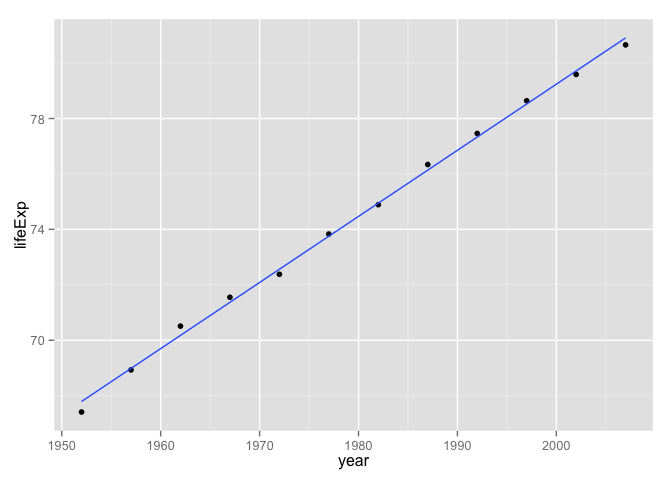

Get some code that works

Fit the regression

j_fit <- lm(lifeExp ~ year, j_dat)
coef(j_fit)
##  (Intercept)         year 
## -397.7646019    0.2385014

Whoa, check out that crazy intercept! Apparently the life expectancy in France around year 0 A.D. was minus 400 years! Never forget to sanity check a model. In this case, a reparametrization is in order. I think it makes more sense for the intercept to correspond to life expectancy in 1952, the earliest date in our dataset. Estimate the intercept eye-ball-o-metrically from the plot and confirm that we’ve got something sane and interpretable now.

j_fit <- lm(lifeExp ~ I(year - 1952), j_dat)
coef(j_fit)
##    (Intercept) I(year - 1952) 
##     67.7901282      0.2385014

Sidebar: regression stuff

There are two things above that might prompt questions.

First, how did I know to get the estimated coefficients from a fitted model via coef()? Years of experience. But how might a novice learn such things? Read the documentation for lm(), in this case. The “See also” section advises us about many functions that can operate on fitted linear model objects, including, but by no means limited to, coef(). Read the documentation on coef() too.

Second, what am I doing here: lm(lifeExp ~ I(year - 1952))? I want the intercept to correspond to 1952 and an easy way to accomplish that is to create a new predictor on the fly: year minus 1952. The way I achieve that in the model formula, I(year - 1952), uses the I() function which “inhibits interpretation/conversion of objects”. By protecting the expression year - 1952, I ensure it is interpreted in the obvious arithmetical way.

Turn working code into a function

Create the basic definition of a function and drop your working code inside. Add arguments and edit the inner code to match. Apply it to the practice data. Do you get the same result as before?

le_lin_fit <- function(dat, offset = 1952) {
  the_fit <- lm(lifeExp ~ I(year - offset), dat)
  coef(the_fit)
}
le_lin_fit(j_dat)
##      (Intercept) I(year - offset) 
##       67.7901282        0.2385014

I had to decide how to handle the offset. Given that I will scale this up to many countries, which, in theory, might have data for different dates, I chose to set a default of 1952. Strategies that compute the offset from data, either the main Gapminder dataset or the excerpt passed to this function, are also reasonable to consider.

I loathe the names on this return value. This is not my first rodeo and I know that, downstream, these will contaminate variable names and factor levels and show up in public places like plots and tables. Fix names early!

le_lin_fit <- function(dat, offset = 1952) {
  the_fit <- lm(lifeExp ~ I(year - offset), dat)
  setNames(coef(the_fit), c("intercept", "slope"))
}
le_lin_fit(j_dat)
##  intercept      slope 
## 67.7901282  0.2385014

Much better!

Test on other data and in a clean workspace

It’s always good to rotate through examples during development. The most common error this will help you catch is when you accidentally hard-wire your example into your function. If you’re paying attention to your informal tests, you will find it creepy that your function returns exactly the same results regardless which input data you give it. This actually happened to me while I was writing this document, I kid you not! I had left j_fit inside the call to coef(), instead of switching it to the_fit. How did I catch that error? I saw the fitted line below, which clearly did not have an intercept in the late 60s and a positive slope, as my first example did. Figures are a mighty weapon in the fight against nonsense. I don’t trust analyses that have few/no figures.

j_country <- "Zimbabwe"
(j_dat <- gapminder %>% filter(country == j_country))
##     country continent year lifeExp      pop gdpPercap
## 1  Zimbabwe    Africa 1952  48.451  3080907  406.8841
## 2  Zimbabwe    Africa 1957  50.469  3646340  518.7643
## 3  Zimbabwe    Africa 1962  52.358  4277736  527.2722
## 4  Zimbabwe    Africa 1967  53.995  4995432  569.7951
## 5  Zimbabwe    Africa 1972  55.635  5861135  799.3622
## 6  Zimbabwe    Africa 1977  57.674  6642107  685.5877
## 7  Zimbabwe    Africa 1982  60.363  7636524  788.8550
## 8  Zimbabwe    Africa 1987  62.351  9216418  706.1573
## 9  Zimbabwe    Africa 1992  60.377 10704340  693.4208
## 10 Zimbabwe    Africa 1997  46.809 11404948  792.4500
## 11 Zimbabwe    Africa 2002  39.989 11926563  672.0386
## 12 Zimbabwe    Africa 2007  43.487 12311143  469.7093
p <- ggplot(j_dat, aes(x = year, y = lifeExp))
p + geom_point() + geom_smooth(method = "lm", se = FALSE)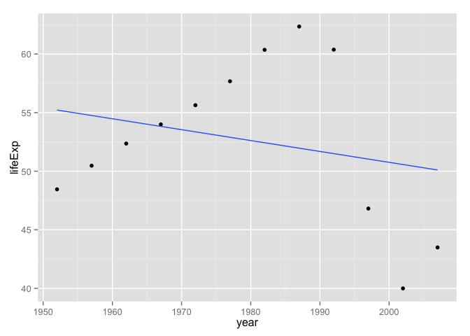

le_lin_fit(j_dat)
##   intercept       slope 
## 55.22124359 -0.09302098

The linear fit is comically bad, but yes I believe the visual line and the regression results match up.

It’s also a good idea to clean out the workspace, rerun the minimum amount of code, and retest your function. This will help you catch another common mistake: accidentally relying on objects that were lying around in the workspace during development but that are not actually defined in your function nor passed as formal arguments.

rm(list = ls())
le_lin_fit <- function(dat, offset = 1952) {
  the_fit <- lm(lifeExp ~ I(year - offset), dat)
  setNames(coef(the_fit), c("intercept", "slope"))
}
le_lin_fit(gapminder %>% filter(country == "Zimbabwe"))
##   intercept       slope 
## 55.22124359 -0.09302098

Are we there yet?

Yes.

Given how I plan to use this function, I don’t feel the need to put it under formal unit tests or put in argument validity checks. Let’s move on to the exciting part, which is scaling this up to all countries.