Unsupervised Learning in Python
- William Surles
- 2017-12-19
- DataCamp class
- https://www.datacamp.com/courses/unsupervised-learning-in-python
Whats Covered
Custering for dataset exploration
- Unsupervised learning
- Evaluating a clustering
- Transforming features for better clusterings
Visualization with hierarchical clustering and t-SNE
- Visualizing hierarchies
- Cluster labels in hierarchical clustering
- t-SNE for 2-dimensional maps
Decorrelating your data and dimension reduction
- Visualizing the PCA transformation
- Intrinsic dimension
- Dimension reduction with PCA
Discovering interpretable features
- Non-negative matrix factorization (NMF)
- NMF learns interpretable parts
- Building recommender systems using NMF
- Final thoughts
Libraries and Data
In [1]:
import pandas as pd
import matplotlib.pyplot as plt
%run data/data.py
Clustering for dataset exploration
Unsupervised learning
Unsupervised learning
- Unspervised learning finds patterns in data
- E.G. clustering customers by their purchases
- Compressing the data using purchase patterns (dimension reduction)
Supervised vs unsupervised learning
- Supervised learning finds paterns for a prediction task
- e.g. classify tumors as benign or cancerous (training on labels)
- Unsupervised learning finds paters in data... but without a specific prediction task in mind
Iris dataset
- measurements of many iris plants
- 3 species of iris: setosa, versicolor, virgininca
- Petal length, petal width, sepal length, wepal width (the features of the dataset)
Arrays, features & samples
- 2D NumPy array
- Columns are measurements (the features)
- Rows represent iris plants (the samples)
Iris data is 4-dimensional
- Iris samples are points in 4 dimensional space
- Dimension = number of features
- Dimension too high to visualize... but unsupervised learning gives insight
k-means clustering
- Finds cluster of samples
- Number of clusters must be specified
- Implemented in
sklearn
Cluster labels for new samples
- new samples can be assigned to existing clusters
- k-means remembers the mean of each cluster (the "centroids")
- Finds the nearest centroid to each new sample
How many clusters?
- 3
In [2]:
xs = points[:,0]
ys = points[:,1]
plt.scatter(xs, ys)
plt.show()

Clustering 2D points
In [3]:
# Import KMeans
from sklearn.cluster import KMeans

# Create a KMeans instance with 3 clusters: model
model = KMeans(n_clusters = 3)

# Fit model to points
model.fit(points)

# Determine the cluster labels of new_points: labels
labels = model.predict(new_points)

# Print cluster labels of new_points
print(labels)
Inspect your clustering
In [4]:
# Import pyplot
import matplotlib.pyplot as plt

# Assign the columns of new_points: xs and ys
xs = new_points[:,0]
ys = new_points[:,1]

# Make a scatter plot of xs and ys, using labels to define the colors
plt.scatter(xs,ys, c=labels, alpha = 0.5)

# Assign the cluster centers: centroids
centroids = model.cluster_centers_

# Assign the columns of centroids: centroids_x, centroids_y
centroids_x = centroids[:,0]
centroids_y = centroids[:,1]

# Make a scatter plot of centroids_x and centroids_y
plt.scatter(centroids_x, centroids_y, marker = 'D', s=50, c = 'k')
plt.show()

Evaluating a clustering
Evaluating a clustering
- Can check correspondence with e.g. iris species ... but what if there are no species to check against?
- We measure quality of a clustering with inertia. This informs choice of how many clusters to look for.
Iris: cluster vs species
- k-means found 3 clusters amongst the iris samples
- Do the clusters correspond to the species?
Cross tabulation with pandas
- Clusters vs species is a "Cross-tabulation"
- Use the pandas library
- Given the species of each sample as a list species
How to evalute a clustering if there were no species information? ...
Measuring clustering quality
- Using only samples and their cluster labels
- A good clusterin has tight clusters ... and samples in each cluster bunched together
Inertia measures clustering quality
- Measures how spread out the clusters are (lower is better)
- Distance from each sample to centroid of its cluster
- After
fit(), available as attributeinertia_ - k_means atempts to minimize the inertia when choosing clusters
How many clusters to choose
- A good clustering has tight clusters (so low inertia) ... but not too many clusters.
- The inertia will keep decreasing as we add more clusters but at some point the decrease will be minimal
- Choose an "elbow" in the inertia plot, where inertia begins to decrease more slowly
How many clusters of grain?
In [5]:
from urllib.request import urlretrieve

url = 'https://archive.ics.uci.edu/ml/machine-learning-databases/00236/seeds_dataset.txt'
urlretrieve(url, 'data/uci_rice')
rice_features = np.loadtxt('data/uci_rice')
print(rice_features.shape)
In [6]:
ks = range(1, 6)
inertias = []

for k in ks:
    # Create a KMeans instance with k clusters: model
    model = KMeans(n_clusters = k)

    # Fit model to samples
    model.fit(rice_features)

    # Append the inertia to the list of inertias
    inertias.append(model.inertia_)

# Plot ks vs inertias
plt.plot(ks, inertias, '-o')
plt.xlabel('number of clusters, k')
plt.ylabel('inertia')
plt.xticks(ks)
plt.show()

Evaluating the grain clustering
In [7]:
rice_names = np.concatenate([np.repeat(name, 70) for name in ['Kama', 'Rosa', 'Canadian']])
rice_names
Out[7]:
In [8]:
# Create a KMeans model with 3 clusters: model
model = KMeans(n_clusters = 3)

# Use fit_predict to fit model and obtain cluster labels: labels
labels = model.fit_predict(rice_features)

# Create a DataFrame with labels and varieties as columns: df
df = pd.DataFrame({'labels': labels, 'varieties': rice_names})

# Create crosstab: ct
ct = pd.crosstab(df['labels'], df['varieties'])

# Display ct
print(ct)
Transforming features for better clusterings
Pidemont wines dataset
- 178 sample from 3 distinct varieties of red wine: Barolo, Grignolino, and Barbera
- Features measure chemical composition e.g. alcohol content
- also visual proerties like " color intensity"
Clustering the wines
In [9]:
file = 'https://assets.datacamp.com/production/course_2072/datasets/wine.csv'
wines = pd.read_csv(file)
wines.head()
Out[9]:
In [10]:
wine_features = wines.drop(['class_label', 'class_name'], axis = 1)
wine_names = wines.class_name
In [11]:
from sklearn.cluster import KMeans
model = KMeans(n_clusters = 3)
labels = model.fit_predict(wine_features)
In [12]:
df = pd.DataFrame({'labels':labels, 'names':wine_names})
ct = pd.crosstab(df['labels'], df['names'])
ct
Out[12]:
Feature variances
- The wine features have very differnet variances
- Variance of a feture measures spread of its values
- especially
prolinewhich has a std of 314
In [13]:
wine_features.describe()
Out[13]:
StandardScaler
- In kmeans: feature variance = feature influence
StandardScalertransforms each feature to have mean o and variance 1- Features are said to be "standardized"
sklearn StandardScaler
In [14]:
from sklearn.preprocessing import StandardScaler

scaler = StandardScaler()

scaler.fit(wine_features)

wine_scaled = scaler.transform(wine_features)

wine_scaled
Out[14]:
Similar methods
- StandardScaler and KMeans have similar methods
- Use
fit()/transform()withStandardScaler - Use
fit()/predict()withKMeans
StandardScaler, then KMeans
- Need to perform tow steps: StandardScaler, then KMeans
- Use sklearn pipeline to combine multiple steps
- Data flows from one step into the next
Pipelines combine multiple steps
In [15]:
from sklearn.preprocessing import StandardScaler
from sklearn.cluster import KMeans
from sklearn.pipeline import make_pipeline

scaler = StandardScaler()
kmeans = KMeans(n_clusters = 3)

pipeline = make_pipeline(scaler, kmeans)

pipeline.fit(wine_features)

labels = pipeline.predict(wine_features)

labels
Out[15]:
Feature standardization improves clustering
- Wow, this is almost perfect now.
In [16]:
df = pd.DataFrame({'labels':labels, 'names':wine_names})
ct = pd.crosstab(df['labels'], df['names'])
ct
Out[16]:
sklearn preprocessing steps
- StandardScaler is a "preprocessing" step
- MaxAbsScaler and Normalizer are other examples
Scaling fish data for clustering
In [17]:
# Perform the necessary imports
from sklearn.pipeline import make_pipeline
from sklearn.preprocessing import StandardScaler
from sklearn.cluster import KMeans

# Create scaler: scaler
scaler = StandardScaler()

# Create KMeans instance: kmeans
kmeans = KMeans(n_clusters = 4)

# Create pipeline: pipeline
pipeline = make_pipeline(scaler, kmeans)
Clustering the fish data
In [18]:
file = 'https://assets.datacamp.com/production/course_2072/datasets/fish.csv'
fish = pd.read_csv(file, header = None)
fish.head()
Out[18]:
In [19]:
fish_features = fish.drop([0], axis = 1)
fish_features.head()
Out[19]:
In [20]:
fish_names = fish[0]
fish_names[0:6]
Out[20]:
In [21]:
# Import pandas
import pandas as pd

# Fit the pipeline to samples
pipeline.fit(fish_features)

# Calculate the cluster labels: labels
labels = pipeline.predict(fish_features)

# Create a DataFrame with labels and species as columns: df
df = pd.DataFrame({'labels': labels,'species': fish_names})

# Create crosstab: ct
ct = pd.crosstab(df['labels'], df['species'])

# Display ct
print(ct)
- But what would it have been without the scaling?
- i.e. what if I de-scale the fish? heh : )
In [22]:
## pipeline with no scaler
pipeline = make_pipeline(kmeans)

pipeline.fit(fish_features)

labels = pipeline.predict(fish_features)

df = pd.DataFrame({'labels': labels,'species': fish_names})

ct = pd.crosstab(df['labels'], df['species'])

print(ct)
- Well, thats not nearly as good. Scaling is legit
Clustering stocks using KMeans
In [23]:
file = 'https://assets.datacamp.com/production/course_2072/datasets/company-stock-movements-2010-2015-incl.csv'
movements = pd.read_csv(file)
movements.head()
Out[23]:
In [24]:
movements_features = movements.drop(['Unnamed: 0'], axis = 1)
movements_names = movements['Unnamed: 0']
In [25]:
# Import Normalizer
from sklearn.preprocessing import Normalizer

# Create a normalizer: normalizer
normalizer = Normalizer()

# Create a KMeans model with 10 clusters: kmeans
kmeans = KMeans(n_clusters = 10)

# Make a pipeline chaining normalizer and kmeans: pipeline
pipeline = make_pipeline(normalizer, kmeans)

# Fit pipeline to the daily price movements
pipeline.fit(movements_features)
Out[25]:
Which stocks move together?
In [26]:
# Import pandas
import pandas as pd

# Predict the cluster labels: labels
labels = pipeline.predict(movements_features)

# Create a DataFrame aligning labels and companies: df
df = pd.DataFrame({'labels': labels, 'companies': movements_names})

# Display df sorted by cluster label
print(df.sort_values('labels'))
Visualization with hierarchical clustering and t-SNE
Visualizing hierarchies
Visualisations communicate insight
- "t-SNE": Creates a 2D map of a dataset (later)
- "Hierarchical clustering" (this video)
A hierarchy of groups
- Groups of living things can form a hierarchy
- Clusters are contained in one another
Hierarchical clustering
- Every country begins in a separate cluster
- At each step, the two closest clusters are merged
- Continue until all countries in a single cluster
- This is "agglomerativer" hierarchical clusting
- There are other ways to do it
How many merges?
- There is always one less merge than there are samples
Hierarchical clustering of the grain data
In [27]:
# Perform the necessary imports
from scipy.cluster.hierarchy import linkage, dendrogram
import matplotlib.pyplot as plt

# Calculate the linkage: mergings
mergings = linkage(rice_features, method = 'complete')

# Plot the dendrogram, using varieties as labels
plt.figure(figsize=(16,10))
dendrogram(
    mergings,
    labels=rice_names.tolist(),
    leaf_rotation=90,
    leaf_font_size=6)
plt.show()

Hierarchies of stocks
In [28]:
# Import normalize
from sklearn.preprocessing import normalize

# Normalize the movements: normalized_movements
normalized_movements = normalize(movements_features)

# Calculate the linkage: mergings
mergings = linkage(normalized_movements, method = 'complete')

# Plot the dendrogram
plt.figure(figsize=(16,10))
dendrogram(
    mergings,
    labels = movements_names.tolist(),
    leaf_rotation = 90,
    leaf_font_size = 10)
plt.show()

Cluster labels in hierarchical clustering
- Not only a visial tool
- Cluster labels at any intermediate stage can be recovered
- Fro use in e.g. cross-tabulations
Dendrograms show cluster distances
- height on dendrogram = distance between merging clusters
- E.G. clusters with only Cyprus and Greece had distance approx. 6
- The new cluster distance approx. 12 from cluster with only Bulgaria
Intermediate clustersing & height on dendrogram
- Height on dendrogram specifies max. distance between merging clusters
- Don't merge clusters further apart than this (e.g. 15)
Distance between clusters
- Defined by a "linkage method"
- Specified via method parameter, e.g.
linkage(samples, method = "complete") - In "complete" linkage: distance between clsuter is max. distance between their samples
- Different linkage method, different hierarchical clustering!
Extracting cluster labels
- Use the
fclustermethod - Returns a NumPy array of cluster labels
Which clusters are closest?
- In complete linkage, the distance between clusters is the distance between the furthest points of the clusters.
- In single linkage, the distance between clusters is the distance between the closest points of the clusters.
Different linkage, different hierarchical clustering!
In [29]:
file = 'https://assets.datacamp.com/production/course_2072/datasets/eurovision-2016.csv'
eurovision = pd.read_csv(file)
eurovision.head()
Out[29]:
In [30]:
eurovision['To country'].nunique()
Out[30]:
In [31]:
eurovision['From country'].nunique()
Out[31]:
In [32]:
eurovision.describe()
Out[32]:
In [33]:
euro_pivot = eurovision.pivot(index = 'From country', columns = 'To country', values = 'Jury Rank')
print(euro_pivot.shape)
euro_pivot.head()
Out[33]:
In [34]:
eurovision_features = euro_pivot.fillna(0)
eurovision_features.head()
Out[34]:
In [35]:
eurovision_names = euro_pivot.index.tolist()
eurovision_names[:6]
Out[35]:
In [36]:
# Perform the necessary imports
import matplotlib.pyplot as plt
from scipy.cluster.hierarchy import linkage, dendrogram

# Calculate the linkage: mergings
mergings = linkage(eurovision_features, method = "single")

# Plot the dendrogram
plt.figure(figsize=(16,10))
dendrogram(
    mergings,
    labels = eurovision_names,
    leaf_rotation = 90,
    leaf_font_size = 12)
plt.show()

This is what it would look like with complete linkage...
In [37]:
# Calculate the linkage: mergings
mergings = linkage(eurovision_features, method = "complete")

# Plot the dendrogram
plt.figure(figsize=(16,10))
dendrogram(
    mergings,
    labels = eurovision_names,
    leaf_rotation = 90,
    leaf_font_size = 12)
plt.show()

Extracting the cluster labels
In [38]:
# Calculate the linkage: mergings
mergings = linkage(rice_features, method = "complete")

# Plot the dendrogram
plt.figure(figsize=(16,10))
dendrogram(
    mergings,
    labels = rice_names,
    leaf_rotation = 90,
    leaf_font_size = 12)
plt.show()

In [39]:
# Perform the necessary imports
import pandas as pd
from scipy.cluster.hierarchy import fcluster

# Use fcluster to extract labels: labels
labels = fcluster(
    mergings,
    8,
    criterion = 'distance')

# Create a DataFrame with labels and varieties as columns: df
df = pd.DataFrame({'labels': labels, 'varieties': rice_names})

# Create crosstab: ct
ct = pd.crosstab(df['labels'],df['varieties'])

# Display ct
print(ct)
t-SNE for 2-dimensional maps
- t-SNE = "t-distributed stochastic neighbor embedding"
- Maps samples to 2D space (or 3D)
- map approximately preserves nearness of samples
- Great for inspecitg datasets
t-SNE has only fit_transform()
- has a
fit_tranform()method - simultaneously fits the model and transforms the data
- Has no separate
fit()ortransoform()methods - Can't extend the map to include new data samples
- Must start over each time!
t-SNE learnign rate
- Choose learning rate for the dataset
- Wrong choice: points bunch together
- Try values between 50 and 200
Different every time
- t-SNE features are different every time
- points will be separated in a similar way but the axis are differnet
t-SNE visualization of grain dataset
In [40]:
classnames, indices = np.unique(rice_names, return_inverse=True)
In [41]:
# Import TSNE
from sklearn.manifold import TSNE

# Create a TSNE instance: model
model = TSNE(learning_rate = 200)

# Apply fit_transform to samples: tsne_features
tsne_features = model.fit_transform(rice_features)

# Select the 0th feature: xs
xs = tsne_features[:,0]

# Select the 1st feature: ys
ys = tsne_features[:,1]

# Scatter plot, coloring by variety_numbers
plt.figure(figsize=(16,10))
plt.scatter(xs, ys, c = indices)
plt.show()

A t-SNE map of the stock market
In [42]:
# Import TSNE
from sklearn.manifold import TSNE

# Create a TSNE instance: model
model = TSNE(learning_rate = 50)

# Apply fit_transform to normalized_movements: tsne_features
tsne_features = model.fit_transform(normalized_movements)

# Select the 0th feature: xs
xs = tsne_features[:,0]

# Select the 1th feature: ys
ys = tsne_features[:,1]

# Scatter plot
plt.figure(figsize=(16,10))
plt.scatter(xs, ys, alpha = .5)

# Annotate the points
for x, y, company in zip(xs, ys, movements_names):
    plt.annotate(company, (x, y), fontsize=10, alpha=0.75)
plt.show()

Decorrelating your data and dimension reduction
Visualizing the PCA transformation
Dimension Reduction
- More efficient storage and computation
- Remove less-informative "noise" features
- ... which cause problems for prediction tasks, e.g. classification, regression
- The instructor says that most prediction problems in the real world are made possible by dimension reduction
Principal Component Analysis
- PCA = "Principal Component Analysis"
- Fundamental dimension reduciton technique
- Most common method of dimension reduction
- First step "decorrelation" (considered here)
- Second step reduces dimension (considered later)
PCA aligns data with axes
- Rotates data samples to be aligned with axes
- Shifts data samples so they have mean 0
- No information is lost
PCA follows the fit/transform pattern
- PCA is a scikit-learn component like KMeans or StandardScaler
fit()learns the transformation from given datatransform()applies the learned transformationtransform()can also be applied to new data
PCA features
- Rows of transformed correspond to samples
- Columns of transformed are the "PCA features"
- Row gives PCA feature values of corresponding sample
PCA features are not correlated
- Features of dataset are often correlated, e.g. total_phenols and od280 (from wine data)
- PCA aligns the data with axes
- Resulting PCA features are not linearly correlated ("decorrelation")
Pearson correlation
- Measures linear correlation of features
- Value between -1 and 1
- Value of 0 means no linear correlation
Principal components
- "Principal components" = directions of variance
- PCA aligns principal components with the axes
- Available as
components_attribute of PCA object - Each row defines displacement from mean
Correlated data in nature
In [43]:
grains = pd.read_csv('data/seeds-width-vs-length.csv', header = None)
grains.head()
Out[43]:
In [44]:
# Perform the necessary imports
import matplotlib.pyplot as plt
from scipy.stats import pearsonr

# Assign the 0th column of grains: width
width = grains.loc[:,0]

# Assign the 1st column of grains: length
length = grains.loc[:,1]

# Scatter plot width vs length
plt.scatter(width, length)
plt.axis('equal')
plt.show()

# Calculate the Pearson correlation
correlation, pvalue = pearsonr(width, length)

# Display the correlation
print(correlation)

Decorrelating the grain measurements with PCA
In [45]:
# Import PCA
from sklearn.decomposition import PCA

# Create PCA instance: model
model = PCA()

# Apply the fit_transform method of model to grains: pca_features
pca_features = model.fit_transform(grains)

# Assign 0th column of pca_features: xs
xs = pca_features[:,0]

# Assign 1st column of pca_features: ys
ys = pca_features[:,1]

# Scatter plot xs vs ys
plt.scatter(xs, ys)
plt.axis('equal')
plt.show()

# Calculate the Pearson correlation of xs and ys
correlation, pvalue = pearsonr(xs, ys)

# Display the correlation
print(correlation)

Intrinsic dimension
Intrinsic dimension of a flight path
- 2 features: longitude and latitude at points along a flight path
- Dataset appears to be 2-dimensional
- But can approximate using one feature: displacement along flight path
- Is intrinsically 1-dimensional
Intrinsic dimension
- Intrinsic dimension = number of features needed to approximate the dataset
- Essential idea behind dimension reduction
- What is the most compact representation of the samples?
- Can be detected with PCA
PCA identifies intrinsic dimension
- Scatter plots work only if samples have 2 or 3 features
- PCA identifies intrinsic dimension when samples have any number of features
- Intrinsic dimension = number of PCA features with significant variance
Variance and intrinsic dimension
- Intrinsic dimension is the number of PCA features with significant variance
- In the versicolor iris example, only the first 2 features
- You can plot the features and see which seem significant
Intrinsic dimension can be ambiguous
- Intrinsic dimension is an idealization
- ... there is not always one correct answer
The first principal component
In [46]:
# Make a scatter plot of the untransformed points
plt.scatter(grains.loc[:,0], grains.loc[:,1])

# Create a PCA instance: model
model = PCA()

# Fit model to points
model.fit(grains)

# Get the mean of the grain samples: mean
mean = model.mean_

# Get the first principal component: first_pc
first_pc = model.components_[0,:]

# Plot first_pc as an arrow, starting at mean
plt.arrow(mean[0], mean[1], first_pc[0], first_pc[1], color='red', width=0.01)

# Keep axes on same scale
plt.axis('equal')
plt.show()

Variance of the PCA features
In [47]:
# Perform the necessary imports
from sklearn.decomposition import PCA
from sklearn.preprocessing import StandardScaler
from sklearn.pipeline import make_pipeline
import matplotlib.pyplot as plt

# Create scaler: scaler
scaler = StandardScaler()

# Create a PCA instance: pca
pca = PCA()

# Create pipeline: pipeline
pipeline = make_pipeline(scaler, pca)

# Fit the pipeline to 'samples'
pipeline.fit(fish_features)

# Plot the explained variances
features = range(pca.n_components_)
plt.bar(features, pca.explained_variance_)
plt.xlabel('PCA feature')
plt.ylabel('variance')
plt.xticks(features)
plt.show()

Intrinsic dimension of the fish data
- 2
Dimension reduction with PCA
Dimension Reduction
- Represents same data, using less features
- Important part of machine-learning pipelines
- Can be performed using PCA
Dimension Reduction with PCA
- PCA features are in decreasing order of variance
- Assumes the low variance features are "noise"
- ... and high variance features are informative
- Specify how many features to keep
- e.g. PCA(n_components=2)
- Keeps the first 2 PCA features
- Intrinsic dimension is a good choice
- Discards low variance PCA features
Word frequency arrays
- Rows represent documents, columns represent words
- Entries measure presence of each word in each document
- ... measure using "tf-idf" (more later)
Sparse arrays and csr_matrix
- Array is "sparse": most entries are zero
- Can use
scipy.sparse.csr_matrixinsted of NumPy array csr_matrixremembers only the non-zero entries (saves space!)
Truncated SVD and csr_matrix
- scikit-learn PCA doesn't support csr_matrix
- Use scikit-learn Truncated SVD instead
- Performs same transformation
Dimension reduction of the fish measurements
In [48]:
# Import PCA
from sklearn.preprocessing import scale
from sklearn.decomposition import PCA

fish_scaled = scale(fish_features)

# Create a PCA model with 2 components: pca
pca = PCA(n_components = 2)

# Fit the PCA instance to the scaled samples
pca.fit(fish_scaled)

# Transform the scaled samples: pca_features
pca_features = pca.transform(fish_scaled)

# Print the shape of pca_features
print(pca_features.shape)
A tf-idf word-frequency array
In [49]:
example_documents = ['cats say meow', 'dogs say woof', 'dogs chase cats']
In [50]:
# Import TfidfVectorizer
from sklearn.feature_extraction.text import TfidfVectorizer

# Create a TfidfVectorizer: tfidf
tfidf = TfidfVectorizer()

# Apply fit_transform to document: csr_mat
csr_mat = tfidf.fit_transform(example_documents)

# Print result of toarray() method
print(csr_mat.toarray())
In [51]:
# Get the words: words
words = tfidf.get_feature_names()

# Print words
print(words)
In [54]:
# Import TfidfVectorizer
from sklearn.feature_extraction.text import TfidfVectorizer

# Create a TfidfVectorizer: tfidf
tfidf = TfidfVectorizer()

# Apply fit_transform to document: csr_mat
csr_mat = tfidf.fit_transform(example_documents)

# Print result of toarray() method
print(csr_mat.toarray())
Clustering Wikipedia part I
In [55]:
import pandas as pd
from scipy.sparse import csr_matrix

df = pd.read_csv('data/wikipedia-vectors.csv', index_col=0)
df.head()
Out[55]:
In [56]:
articles = csr_matrix(df.transpose())
titles = list(df.columns)
In [57]:
# Perform the necessary imports
from sklearn.decomposition import TruncatedSVD
from sklearn.cluster import KMeans
from sklearn.pipeline import make_pipeline

# Create a TruncatedSVD instance: svd
svd = TruncatedSVD(n_components = 50)

# Create a KMeans instance: kmeans
kmeans = KMeans(n_clusters = 6)

# Create a pipeline: pipeline
pipeline = make_pipeline(svd, kmeans)
Clustering Wikipedia part II
In [58]:
# Import pandas
import pandas as pd

# Fit the pipeline to articles
pipeline.fit(articles)

# Calculate the cluster labels: labels
labels = pipeline.predict(articles)

# Create a DataFrame aligning labels and titles: df
df = pd.DataFrame({'label': labels, 'article': titles})

# Display df sorted by cluster label
print(df.sort_values('label'))
- Wow, that so simple of a pipeline, and it does such a good job of clustering
- These groups totally makes sense. I love this.
Discovering interpretable features
Non-negative matrix factorization (NMF)
Non-negative matrix factorization
- NMF = "non-negative matrix factorization"
- Dimension reduction technique
- NMF models are interpretable (unlike PCA)
- Easy to interpret means easy to explain!
- However, all samples features must be non-negative (>= 0)
Interpretable parts
- NMF expresses documents as combinations of topics (or "themes")
- NMF expresses images as combinations of patterns
Using scikit-learn NMF
- Follows
fit()/transform()pattern - Must specify number of components e.g.
NMF(n_components = 2) - Works with NumPy arrays and with
csr_matrix
Example word-frequency array
- Word frequency array, 4 words, many documents
- Measure presence of words in each document using "tf-idf"
- "tf" - frequency of word in document
- "idf" - reduces influence of frequent words
NMF components
- NMF has components... just like pcA has principal components
- Dimension of components = dimension of samples
- Entries are non-negative
NMF features
- NMF feature values are non-negative
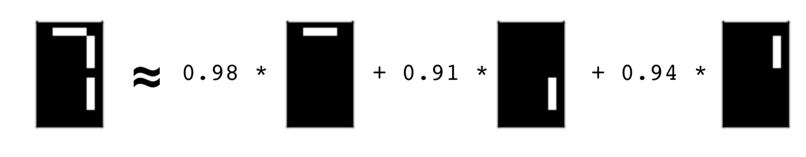
- Can be used to reconstruct the samples
- ... combine feature values with components
Sample reconstruction
- Multiply components by feature values, and add up
- Can also be expressed as a product of matrices
- This is the "Matrix Factorization" in "NMF"
NMF fits to non-negative data only
- Word frequencies in each document
- Images encoded as arrays
- Audio spectrograms
- Purchase histories on e-commerce sites
- ... and many more
NMF applied to Wikipedia articles
In [59]:
# Import NMF
from sklearn.decomposition import NMF

# Create an NMF instance: model
model = NMF(n_components = 6)

# Fit the model to articles
model.fit(articles)

# Transform the articles: nmf_features
nmf_features = model.transform(articles)

# Print the NMF features
print(nmf_features[:6])
NMF features of the Wikipedia articles
In [60]:
# Import pandas
import pandas as pd

# Create a pandas DataFrame: df
df = pd.DataFrame(nmf_features, index = titles)
df.head()
Out[60]:
In [61]:
# Print the row for 'Anne Hathaway'
print(df.loc['Anne Hathaway'])

# Print the row for 'Denzel Washington'
print(df.loc['Denzel Washington'])
- Notice that for both actors, the NMF feature 3 has by far the highest value.
- This means that both articles are reconstructed using mainly the 3rd NMF component.
- In the next video, you'll see why: NMF components represent topics (for instance, acting!).
NMF learns interpretable parts
Example: NMF learns interpretable parts
- Word-frequency array
articles(tf-idf) - 20,000 scientific articles(rows)
- 800 words (columns)
- apply NMF with number of components
- the components will be topics
- You can see the top words for a topic
Example: NMF learns images
- "Grayscale" image = no colors, only shades of gray
- Measure pixel brighness
- Represent with value between 0 and 1 (0 is black)
- Convert to 2D array
- Flateen to 1D array
- enumerate the entries by row left to right into array
- Collection of images of same size
- for collection of images each row will be an image
- each column will be a specific pixel
- The components will be parts of the images
NMF learns topics of documents
In [62]:
words = pd.read_csv('data/wikipedia-vocabulary-utf8.txt', header = None)[0]
words[:6]
Out[62]:
In [63]:
# Import pandas
import pandas as pd

# Create a DataFrame: components_df
components_df = pd.DataFrame(model.components_, columns = words)
components_df.head()
Out[63]:
In [64]:
# Print the shape of the DataFrame
print(components_df.shape)
In [65]:
# Select row 3: component
component = components_df.iloc[3,:]

# Print result of nlargest
print(component.nlargest(20))
Explore the LED digits dataset
In [66]:
file = 'https://assets.datacamp.com/production/course_2072/datasets/lcd-digits.csv'
digits = pd.read_csv(file, header = None).as_matrix()
digits
Out[66]:
In [67]:
# Import pyplot
from matplotlib import pyplot as plt

# Select the 0th row: digit
digit = digits[0,:]

# Print digit
print(digit)
In [68]:
# Reshape digit to a 13x8 array: bitmap
bitmap = digit.reshape(13,8)

# Print bitmap
print(bitmap)
In [69]:
# Use plt.imshow to display bitmap
plt.imshow(bitmap, cmap='gray', interpolation='nearest')
plt.colorbar()
plt.show()

NMF learns the parts of images
In [70]:
# Import NMF
import matplotlib.pyplot as plt
from sklearn.decomposition import NMF

# Create an NMF model: model
model = NMF(n_components = 7)

# Apply fit_transform to samples: features
features = model.fit_transform(digits)

# Call show_as_image on each component
plt.figure(figsize=(18,10))
x = 1
for component in model.components_:
    bitmap = component.reshape(13,8)
    plt.subplot(2,4,x)
    plt.imshow(bitmap, cmap='gray', interpolation='nearest')
    x += 1

plt.show()

In [71]:
# Assign the 0th row of features: digit_features
digit_features = features[0,:]

# Print digit_features
print(digit_features)
- If you put the 1, 4 and 5 images together you get a seven. Cool
PCA doesn't learn parts
- Red means a negative value
- basically all the components have most of the parts
In [72]:
def show_as_image(vector, x):
    """
    Given a 1d vector representing an image, display that image in
    black and white.  If there are negative values, then use red for
    that pixel.
    """
    bitmap = vector.reshape((13, 8))  # make a square array
    bitmap /= np.abs(vector).max()  # normalise
    bitmap = bitmap[:,:,np.newaxis]
    rgb_layers = [np.abs(bitmap)] + [bitmap.clip(0)] * 2
    rgb_bitmap = np.concatenate(rgb_layers, axis=-1)

    plt.subplot(2,4,x)
    plt.imshow(rgb_bitmap, interpolation='nearest')
    plt.xticks([])
    plt.yticks([])
In [73]:
# Import PCA
from sklearn.decomposition import PCA

# Create a PCA instance: model
model = PCA(n_components = 7)

# Apply fit_transform to samples: features
features = model.fit_transform(digits)

# Call show_as_image on each component
plt.figure(figsize=(18,10))
x = 1
for component in model.components_:
    show_as_image(component, x)
    x += 1
plt.show()

Building recommender systems using NMF
Finding similar articles
- Engineer at a large online newspaper
- Task: recommend articles similar to article being read by customer
- Similar articles should have similar topics
Strategy
- Apply NMF to the word-frequency array
- NMF feature values describe the topics
- ... so similar documetns have similar NMF feature values
- Compare NMF feature values?
Versions of articles
- Different versions of the same document have same topic proportions
- ... exact feature values may be different
- e.g. because one version uses many meaningless words (weaker language)
- But all versions lie on the same line through the origin
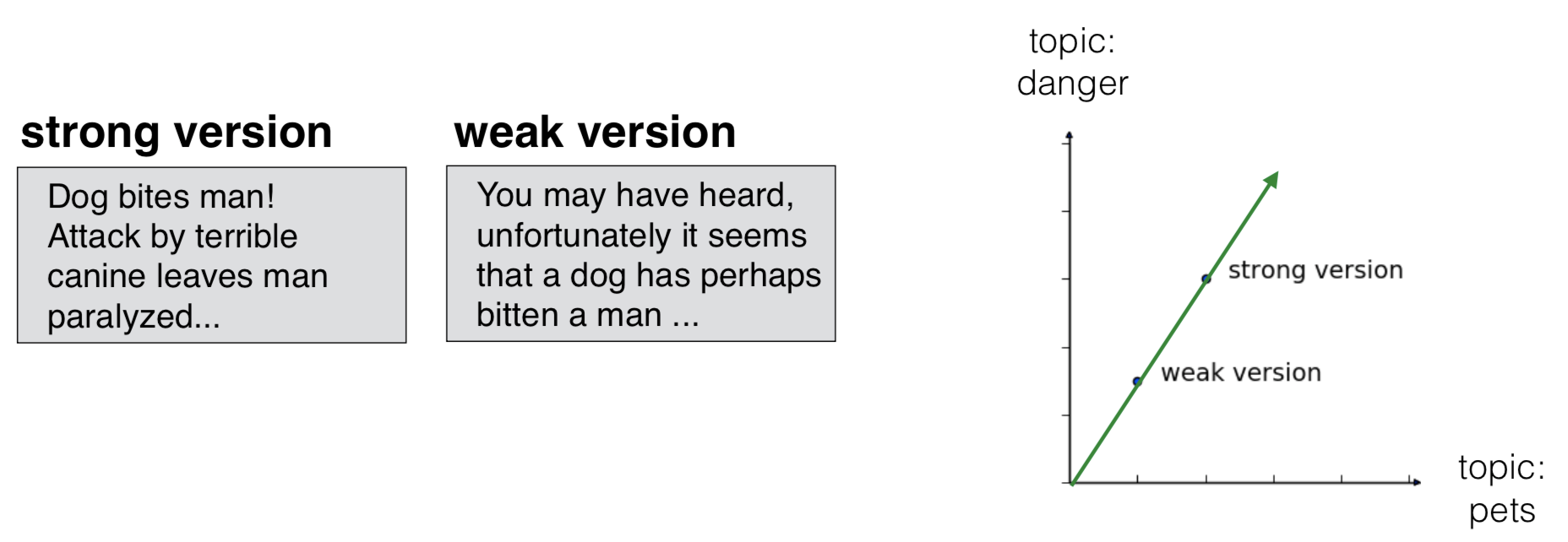
Cosine similarity
- Uses the angle between the lines
- Higher vaues mean more similar
- maximum value is 1, when angle is 0 deg
Which articles are similar to 'Cristiano Ronaldo'?
In [74]:
# Perform the necessary imports
import pandas as pd
from sklearn.preprocessing import normalize

# Normalize the NMF features: norm_features
norm_features = normalize(nmf_features)

# Create a DataFrame: df
df = pd.DataFrame(norm_features, index = titles)

# Select the row corresponding to 'Cristiano Ronaldo': article
article = df.loc['Cristiano Ronaldo']

# Compute the dot products: similarities
similarities = df.dot(article)

# Display those with the largest cosine similarity
print(similarities.nlargest(10))
Recommend musical artists part I
Load artist data and get it in the right shape for the exercise
In [75]:
file = 'data/scrobbler-small-sample.csv'
artists = pd.read_csv(file)
artists.head()
Out[75]:
In [76]:
artists.shape
Out[76]:
- we want the user listens for each artist.
- Topics will be users and scores will be listens I guess.
- So we need to pivot
- You could think of this as the sparse document matrix where articles are the rows and words are the columns
In [77]:
artists_spread = artists.pivot(
    index = 'artist_offset',
    columns = 'user_offset',
    values = 'playcount'
    ).fillna(0)
artists_spread.head()
Out[77]:
In [78]:
artists_spread.shape
Out[78]:
In [79]:
## load the corresponding artist names
file = 'data/artists.csv'
artists_names = pd.read_csv(file, header = None)[0].tolist()
artists_names[:6]
Out[79]:
Exercise
In [80]:
# Perform the necessary imports
from sklearn.decomposition import NMF
from sklearn.preprocessing import Normalizer, MaxAbsScaler
from sklearn.pipeline import make_pipeline

# Create a MaxAbsScaler: scaler
scaler = MaxAbsScaler()

# Create an NMF model: nmf
nmf = NMF(n_components = 20)

# Create a Normalizer: normalizer
normalizer = Normalizer()

# Create a pipeline: pipeline
pipeline = make_pipeline(scaler, nmf, normalizer)

# Apply fit_transform to artists: norm_features
norm_features = pipeline.fit_transform(artists_spread)
In [81]:
norm_features.shape
Out[81]:
Recommend musical artists part II
In [82]:
# Import pandas
import pandas as pd

# Create a DataFrame: df
df = pd.DataFrame(norm_features, index = artists_names)
df.head()

# Select row of 'Bruce Springsteen': artist
artist = df.loc['Bruce Springsteen']

# Compute cosine similarities: similarities
similarities = df.dot(artist)

# Display those with highest cosine similarity
print(similarities.nlargest(10))
Final thoughts
- This class was simple and to the point
- I can't belive its that easy to make a recommendation system
- I know there will be lost more details to consider in the real world but still
- Great class