Querying Twitter Data
Ryan Wesslen
July 20, 2017
Objective: Keyword Search for Panther Tweets
Our goal is to learn how to find and analyze specific Tweets: Carolina Panther Tweets. Along the way, we’ll analyze what Panther fans are saying and, related, explore where they Tweet from through geo-location.
The dataset we’ll use is a 20% sample of all Charlotte geo-located Tweets in a three month period (Dec 1 2015 to Feb 29 2016). The dataset is 47,274 Tweets and includes 18 columns on information about the Tweet and the User who posted the Tweet.
There are two ways to run this file: as automatically as a Knit (e.g. to produce a HTML file) or in manually chunks.
If you run it in chunks (as we will in this tutorial), you will need to set your working directory and remove one of the “.” from the read.csv() and source() functions. If you are running it as Knit file, you can leave as is.
Step 1: Read in the data.
library(tidyverse)

file <- "../data/CharlotteTweets20Sample.csv"
#file <- "~/Dropbox (UNC Charlotte)/summer-2017-social-media-workshop/data/CharlotteTweets20Sample.csv"
raw.tweets <- read_csv(file)
Step 2: Explore the dataset.
Let’s explore our dataset. You can either open the dataset or run the str() function.
str(raw.tweets)## Classes 'tbl_df', 'tbl' and 'data.frame': 47274 obs. of 18 variables:
## $ body : chr "Treon to WR is a really good move by Mac, very familiar with playbook. Very good runner in open space too" "primus #vsco #vscocam #primus #primussucks #charlotte #bojanglescoliseum #livemusic… https://t.co/IqI6BIPVqn" "WOAH!!!!!!" "clear -> mostly cloudytemperature down 59°F -> 54°Fhumidity up 88% -> 100%visibility 10mi -> 5mi" ...
## $ postedTime : POSIXct, format: "2016-02-05 17:23:34" "2016-01-28 00:20:32" ...
## $ actor.id : num 3.86e+08 1.55e+07 9.10e+07 2.25e+08 7.73e+07 ...
## $ displayName : chr "Clint Lawrence" "Josh Hofer" "hector vargas #28" "Kannapolis Weather" ...
## $ actor.postedTime : POSIXct, format: "2011-10-06 17:28:32" "2008-07-19 16:49:51" ...
## $ summary : chr "Follower of Jesus Christ, husband, father, trains like a boss and LOVE all UF sports" "Photographer {http://www.flickr.com/corruptedlens} || Music. || n3rd. || iPhone. || Instagram {http://instagram.com/josh_hofer}"| __truncated__ "Proud Dad, Die Hard Mets fan. Transplant New Yorker in NC. Love the GMEN and Knicks basketball #The7lineArmy" "Weather updates, forecast, warnings and information for Kannapolis, NC. Sources: Yahoo! Weather, NOAA, USGS." ...
## $ friendsCount : int 617 692 1241 2 1886 144 131 501 270 825 ...
## $ followersCount : int 257 1204 268 70 1923 388 1279 479 97 3813 ...
## $ statusesCount : int 3447 16235 22645 20292 22428 162 15196 4791 5508 27450 ...
## $ actor.location.displayName: chr "Fort Mill, SC" "Raleigh, NC" "Huntersville, NC" "Kannapolis, NC" ...
## $ generator.displayName : chr "Twitter for iPhone" "Instagram" "Tweetbot for iΟS" "Cities" ...
## $ geo.type : chr "Polygon" "Point" "Polygon" "Point" ...
## $ point_long : num NA 35.2 NA 35.5 NA ...
## $ point_lat : num NA -80.8 NA -80.6 NA ...
## $ urls.0.expanded_url : chr NA "https://www.instagram.com/p/BBD_iFMJMQb/" NA NA ...
## $ klout_score : int 41 52 38 19 49 41 48 41 38 59 ...
## $ hashtags : chr NA "vsco,vscocam,primus,primussucks,charlotte,bojanglescoliseum,livemusic" NA NA ...
## $ user_mention_screen_names : chr NA NA NA NA ...
## - attr(*, "spec")=List of 2
## ..$ cols :List of 18
## .. ..$ body : list()
## .. .. ..- attr(*, "class")= chr "collector_character" "collector"
## .. ..$ postedTime :List of 1
## .. .. ..$ format: chr ""
## .. .. ..- attr(*, "class")= chr "collector_datetime" "collector"
## .. ..$ actor.id : list()
## .. .. ..- attr(*, "class")= chr "collector_double" "collector"
## .. ..$ displayName : list()
## .. .. ..- attr(*, "class")= chr "collector_character" "collector"
## .. ..$ actor.postedTime :List of 1
## .. .. ..$ format: chr ""
## .. .. ..- attr(*, "class")= chr "collector_datetime" "collector"
## .. ..$ summary : list()
## .. .. ..- attr(*, "class")= chr "collector_character" "collector"
## .. ..$ friendsCount : list()
## .. .. ..- attr(*, "class")= chr "collector_integer" "collector"
## .. ..$ followersCount : list()
## .. .. ..- attr(*, "class")= chr "collector_integer" "collector"
## .. ..$ statusesCount : list()
## .. .. ..- attr(*, "class")= chr "collector_integer" "collector"
## .. ..$ actor.location.displayName: list()
## .. .. ..- attr(*, "class")= chr "collector_character" "collector"
## .. ..$ generator.displayName : list()
## .. .. ..- attr(*, "class")= chr "collector_character" "collector"
## .. ..$ geo.type : list()
## .. .. ..- attr(*, "class")= chr "collector_character" "collector"
## .. ..$ point_long : list()
## .. .. ..- attr(*, "class")= chr "collector_double" "collector"
## .. ..$ point_lat : list()
## .. .. ..- attr(*, "class")= chr "collector_double" "collector"
## .. ..$ urls.0.expanded_url : list()
## .. .. ..- attr(*, "class")= chr "collector_character" "collector"
## .. ..$ klout_score : list()
## .. .. ..- attr(*, "class")= chr "collector_integer" "collector"
## .. ..$ hashtags : list()
## .. .. ..- attr(*, "class")= chr "collector_character" "collector"
## .. ..$ user_mention_screen_names : list()
## .. .. ..- attr(*, "class")= chr "collector_character" "collector"
## ..$ default: list()
## .. ..- attr(*, "class")= chr "collector_guess" "collector"
## ..- attr(*, "class")= chr "col_spec"Step 3: Run time series plot of Tweets.
Run the functions.R file with pre-created functions. We’ll use the source() function to run the file.
To run a time series plot of the dataset, use the timePlot() function. [The plot uses the packages ggplot2. You can open the functions file to see the steps used to create the plot if you’re interested.]
Add the parameter “smooth = TRUE” to add a smoothing parameter.
#remove one of the "." if you are running as chunks
#source("~/Dropbox (UNC Charlotte)/summer-2017-social-media-workshop/day2/querying-functions.R")
source("./querying-functions.R")

#pre-created function in the functions.R file
timePlot(raw.tweets, smooth = TRUE)
Note the spikes. What is causing the spikes?
Step 5: Hashtag Keywords
From this analysis, we’ve identified three key hashtag/handles that are related to the panthers: #KeepPounding, #Panthers and @Panthers.
Let’s find all of the tweets in our original dataset that contain these hashtags/handles.
To accomplish this, we need to use a regular expression grepl() that will identify any tweets that include these hashtags/handles. For an overview of regular expression in R, see this tutorial. We’ll discuss more about regular expressions in tomorrow’s workshop.
First, let’s save the hashtags and handles into a character vector: names <- c(“keyword1”,“keyword2”)
panthers <- c("#keeppounding", "#panthers", "@panthers")Now let’s use the grepl() function to identify any tweets that include our keywords.
First, to combine all of the keywords, we’ll use paste(names, collapse = "|") to create a string of the keywords (with | as an OR).
Second, we’ll use the tolower() function that converts all of the Tweets to lower case. This is helpful as it ignores lower case.
# find only the Tweets that contain words in the first list
hit <- grepl(paste(panthers, collapse = "|"), raw.tweets$body, ignore.case = TRUE)
Then, let’s go back to our original dataset and select only the rows that meet our criteria. After, let’s count the number of rows we have using this criteria.
# create a dataset with only the tweets that contain these words
panther.tweets <- raw.tweets[hit,]

nrow(panther.tweets)
## [1] 1113Using this criteria, we find 1,113 Tweets. Let’s plot the time series:
timePlot(panther.tweets)
As a comparison, let’s plot our original dataset but removing our Panther Tweets:
nonpanther.tweets <- raw.tweets[-hit,]

timePlot(nonpanther.tweets)
The problem is we still see some of the spikes, which implies that we’re missing some Panther tweets. This makes sense as it’s possible that some Panther-related Tweets do not necessarily include the hashtags we’ve identified.
Step 6: Text Analysis with quanteda
For this exercise, we need to expand our list of Panther keywords beyond our initial set of hashtags and handles.
To accomplish this goal, let’s create word clouds to examine the common words used in the Panther-related Tweets we’ve identified. We will use the quanteda package
library(quanteda); library(RColorBrewer)The quanteda package allows you to take a text (character) column and convert it into a DFM (data feature matrix, a generalization of a document-term matrix).
To do this, first, we have to use the corpus function to create our corpus. The corpus is data object that specializes in handling sparse (text) data.
MyCorpus <- corpus(panther.tweets$body)You can retrieve any of the documents by using the following command:
MyCorpus$documents[[1]][1]## [1] "NFC Champs, Super Bowl bound. #KeepPounding @ Bank of America Stadium https://t.co/6bEWkbsAjQ"With our corpus, let’s now create the dfm object. This step facilitates data pre-processing steps including removing stop words (words with little meaning) with the ignoredFeature parameter. We can also expand beyond considering single word terms to consider two-word terms (bigrams) by using the ngrams parameter.
dfm <- dfm(MyCorpus,
           remove = c(stopwords("english"), "t.co", "https", "rt", "amp", "http", "t.c", "can", "u"),
           remove_numbers = TRUE,
           remove_punct = TRUE,
           remove_symbols = TRUE,
           ngrams=1L)
Let’s look at the first Tweet and 10 terms.
dfm_sort(dfm)[1,1:10]## Document-feature matrix of: 1 document, 10 features (50% sparse).
## 1 x 10 sparse Matrix of class "dfmSparse"
## features
## docs #keeppounding @panthers #panthers bank america stadium panthers
## text1 1 0 0 1 1 1 0
## features
## docs #panthernation go super
## text1 0 0 1With our dfm, let’s view our top 25 terms in our corpus, using the topfeatures() function.
topfeatures(dfm,25)## #keeppounding @panthers #panthers bank
## 732 341 184 148
## america stadium panthers #panthernation
## 129 127 121 87
## go super bowl game
## 83 76 73 73
## charlotte carolina #panthersnation win
## 69 50 49 49
## #carolinapanthers #gopanthers #charlotte see
## 47 37 36 36
## time just love day
## 35 30 29 29
## will
## 29Not surprising, the most common terms include our hashtags. But what’s interesting is the "@", “bank”, “america”, “stadium” are the next most common terms. It appears that people are using “@ Bank of America Stadium” but the problem is that during the tokenization (during pre-processing) the spaces make the term to appear as different terms. We will ignore this for now but the ultimate cause is that Instagram and Facebook have the BofA stadium appear as “@ Bank of America Stadium”. [Question - how could we correct this in pre-processing now that we know this?]
But what’s clear is that there are other terms that appear to relevant: e.g. #carolinapanthers, #panthersnation, #gopanthers. Already, we now know that we’re missing some Panther hashtags.
Let’s consider what are all the words in these panther tweets by using a word cloud:
textplot_wordcloud(dfm,
                   scale=c(3.5, .75),
                   colors=brewer.pal(8, "Dark2"),
                   random.order = F,
                   rot.per=0.1,
                   max.words=100)
One further analysis we can to calculate the similarity between words to identify other Panther keywords.
simil <- textstat_simil(dfm, c("keeppounding", "panthers"), method = "cosine", margin = "features")
simil <- simil[order(simil, decreasing = TRUE),]

head(as.matrix(simil), n = 10)
## [,1]
## panthers 1.0000000
## #sbvote 0.4489436
## @sportscenter 0.4405514
## taking 0.4326129
## win 0.3209498
## #keeppounding 0.3131053
## bowl 0.3110437
## super 0.3051560
## go 0.3020616
## ylatvyisaa 0.1760902Step 7: Advanced Panthers Keywords
Already, we’ve seen that are simple list of initial Panther hashtags/handles is insufficient.
A key lesson is that there is almost never a perfect list of keywords to use! That’s why asking the question “is this all of the Tweets related to a topic” is a very “loaded” question.
After running through a few iterations, I found an advanced list of keywords that expand our list of Panther tweets. Let’s rerun our analysis but using these keywords instead.
panthers <- c("panther","keeppounding","panthernation","CameronNewton","LukeKuechly",
              "cam newton ","thomas davis","greg olsen","kuechly","sb50","super bowl",
              "sbvote","superbowl","keep pounding","camvp","josh norman")

# find only the Tweets that contain words in the first list
hit <- grepl(paste(panthers, collapse = "|"), tolower(raw.tweets$body))

# create a dataset with only the tweets that contain these words
panther.tweets <- raw.tweets[hit,]

nrow(panther.tweets)
## [1] 2048timePlot(panther.tweets)
So now we have 2,048 Tweets, instead of our original 1,113 Tweets – nearly doubling our original count.
Let’s rerun our text analysis steps but this time we’re going to add in the column geo.type. This column indicates whether the Tweet was a point or a polygon.
To do this, we will add the field using the docvars() function to our corpus.
MyCorpus <- corpus(panther.tweets$body)
docvars(MyCorpus) <- data.frame(geo.type=panther.tweets$geo.type)

dfm <- dfm(MyCorpus,
           remove = c(stopwords("english"), "t.co", "https", "rt", "amp", "http", "t.c", "can", "u"),
           remove_numbers = TRUE,
           remove_punct = TRUE,
           remove_symbols = TRUE,
           ngrams=1L)

topfeatures(dfm)
## #keeppounding panthers @panthers bank stadium
## 732 572 341 218 194
## super america #panthers bowl carolina
## 192 191 184 182 164textplot_wordcloud(dfm,
scale=c(3.5, .75),
colors=brewer.pal(8, "Dark2"),
random.order = F,
rot.per=0.1,
max.words=100)
Step 8: Comparison Word Cloud by Geolocation Type
Now, let’s use our geo.type field to compare the words being used
Rerun the dfm but this time add in the geo.type as a group. Run a comparison word cloud (comparison = TRUE). This may take a few minutes.
pnthrdfm <- dfm(MyCorpus,
                groups = "geo.type",
                remove = c(stopwords("english"), "t.co", "https", "rt", "amp", "http", "t.c", "can", "u"),
                remove_numbers = TRUE,
                remove_punct = TRUE,
                remove_symbols = TRUE,
                ngrams=1L)

textplot_wordcloud(pnthrdfm,
                   comparison = TRUE,
                   scale=c(3.5, .75),
                   colors=brewer.pal(8, "Dark2"),
                   random.order = F,
                   rot.per=0.1,
                   max.words=100)
What appears to be the difference in the types of geo-located tweets?
Let’s dig further by plotting the time series of each Tweet type using the timePlot() function:
timePlot(panther.tweets[panther.tweets$geo.type == "Point",], smooth = FALSE)
timePlot(panther.tweets[panther.tweets$geo.type == "Polygon",], smooth = FALSE)
Let’s use the leaflet package to plot the points. (Note: for some reason, I had problems running this on my Mac. Not sure. Let me know if you experience the same issue.)
library(leaflet) #run if you do not have it already, install.packages("leaflet")

t <- subset(panther.tweets, geo.type == "Point")

# fyi the lat and long columns are mislabelled
leaflet() %>%
  addTiles() %>%
  addCircleMarkers(lng=t$point_lat, lat=t$point_long,   popup = t$body, #color = pal(points$generator),
             stroke = FALSE, fillOpacity = 0.5, radius = 10, clusterOptions = markerClusterOptions()
             )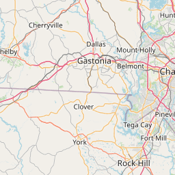
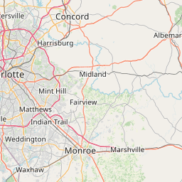
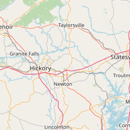
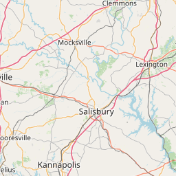
Where are most of the point Tweets? Of course close to the stadium.
Bonus - Additional Pre-Processing Steps
There are also additional pre-processing steps can sometimes improve results. Run additional pre-processing steps including: stemming, Twitter mode, bigrams or trigrams. Use ?dfm help to get a list of the parameters.
dfm <- dfm(MyCorpus,
           remove = c(stopwords("english"), "t.co", "https", "rt", "amp", "http", "t.c", "can", "u"),
           stem = TRUE,
           remove_numbers = TRUE,
           remove_punct = TRUE,
           remove_symbols = TRUE,
           remove_twitter = TRUE,
           ngrams=1L)

topfeatures(dfm)
## panther keeppound bank stadium charlott super america
## 1205 776 218 195 195 193 191
## go bowl carolina
## 188 186 185textplot_wordcloud(dfm, scale=c(3.5, .75), colors=brewer.pal(8, "Dark2"),
random.order = F, rot.per=0.1, max.words=100)
What are the differences between this plot and our original plots? Is it worth it to use these pre-processing steps?
We’ll discuss more in the next workshop about why it may be helpful to use these steps sometimes in text analysis.