

The Cell Profiler
Abstract: (Click to View Original Proposal)
Identifying and counting cells in images is the first stage of cell analysis, but this step can become extraordinarily time consuming if done manually as the number of cells and organisms increase. Our goal was to take a micrograph, a magnified image containing cells taken through a microscope lens, and return information about cell type and number. For this, we implemented two models. In our first model, we trained a high level image classifier followed by class specific detection algorithms and finally evaluated the metrics. Our second approach involves a generic cell detector, followed by classification. We have compared the performance of both these models in terms of precision, recall and mean RMS cell-count error. We used two data-sets: C.elegans and Human Bone Osteosarcoma Epithelial Cells (U2OS Line), that provide ground truth segmentation of cells.


Introduction
Data Sets
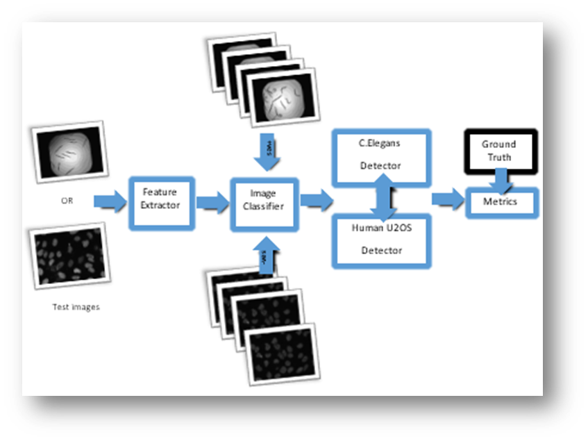
Figure1: Approach 1
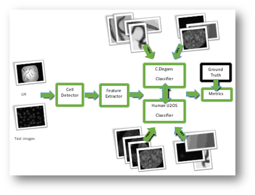
Figure2: Approach 2
Classifier
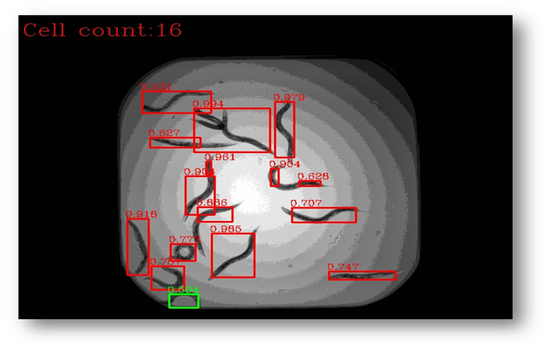
C-Elegans Detector [Approach 1]
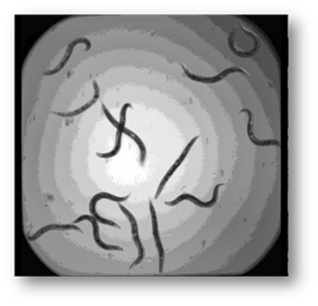
Figure3: Input image
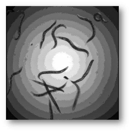
Figure4: Input image example where the C. Elegans blend into the background
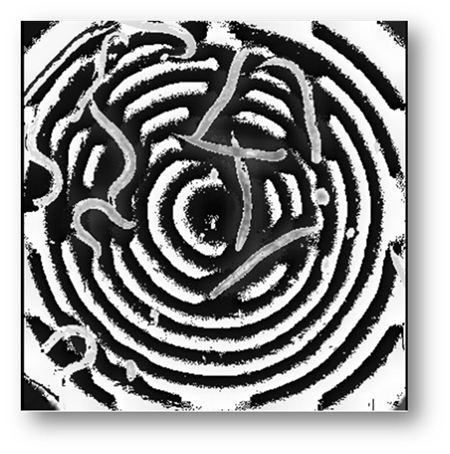
Figure5: Background subtracted image
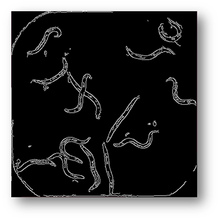
Figure6: Image processed using canny edge detection


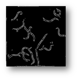
Figure7(a,b,c): Showing the process of removing the borders
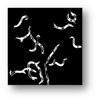
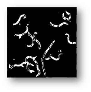
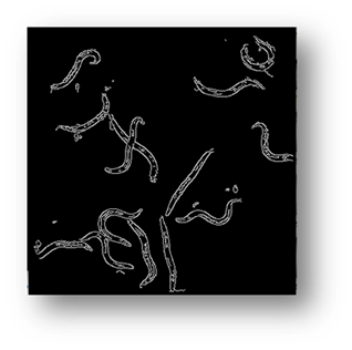
Figure8(a,b,c): Showing the results of filtering the small components out of the image
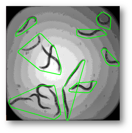
Figure9: The results of using the external contour connection based on distance method
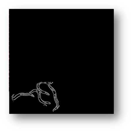

Figure10(a,b): Showing the process and result of masking for counting pixels for cell number estimation
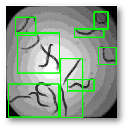
Figure11: The final result with bounding boxes
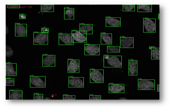
Human U2OS Detector [Approach 1]
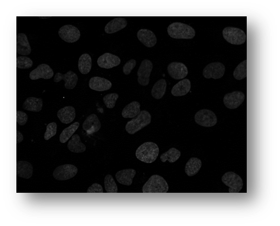
Figure12: Microscopic image of U2OS cancer cells.
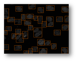
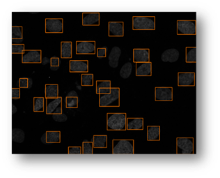
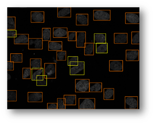
Figure13(a,b,c): Shows the advantage of using an iterative thresholding approach. (a) shows a low threshold value and it does not separate all of the cells. (b) shows a high threshold value and it misses some cells and thinks other cells are smaller than they really are. (c) shows an iterative approach starting from the lower threshold value in (a) and moving to the value in (c) and evaluates at each step to see if the segmentation is better. Additional segmentations between (a) and (c) are shown in yellow in (c).
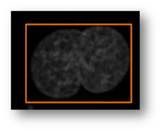
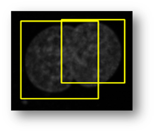
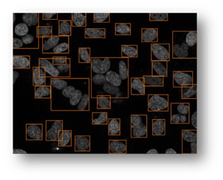
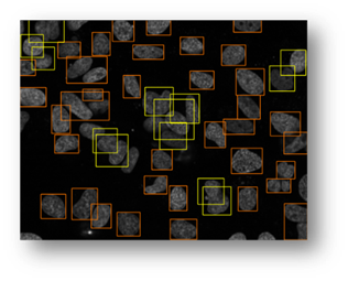
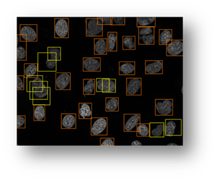
Figure14(a,b,c,d,e): Segmented images displaying the results of circle detection segmentations shown in yellow. (b) shows a successful segmentation of the cell shown in (a) that could not be separated by the connected components technique. (d) shows the method successfully implemented on (c) while (e) is a failure case of the circle detection method for cell separation.
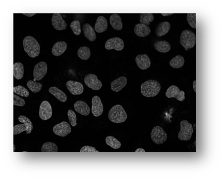
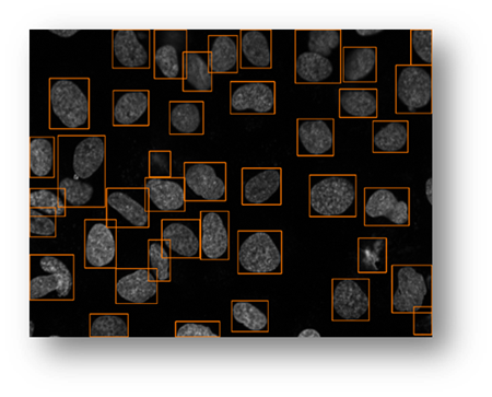
Figure15(a,b): Example input and output of final algorithm to segment U2OS cells.
Generic Detector [Approach 2]
Results
Figure16
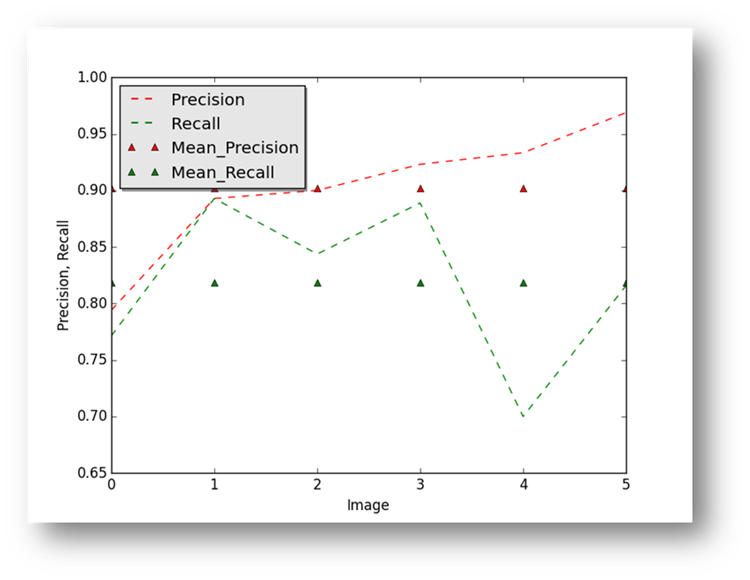
Figure17
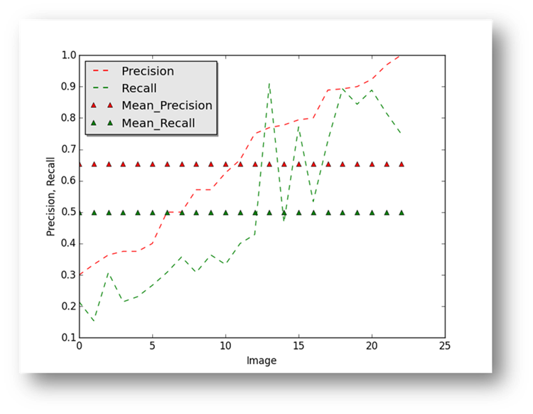
Figure18
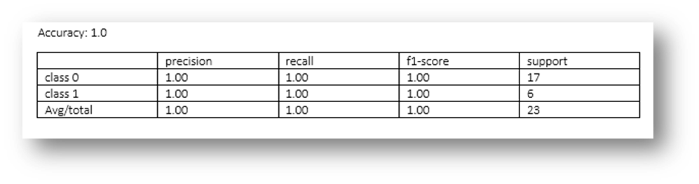
Figure19
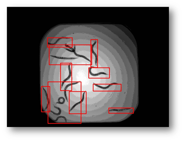
Figure20
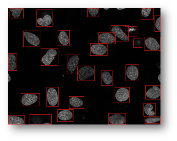
Figure21
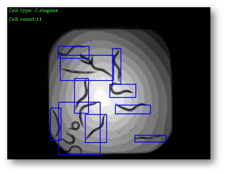
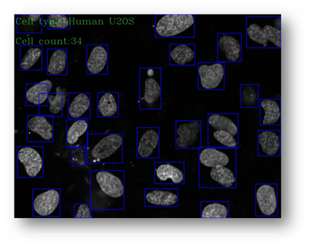
Figure22(a,b)
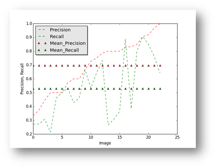
Figure23
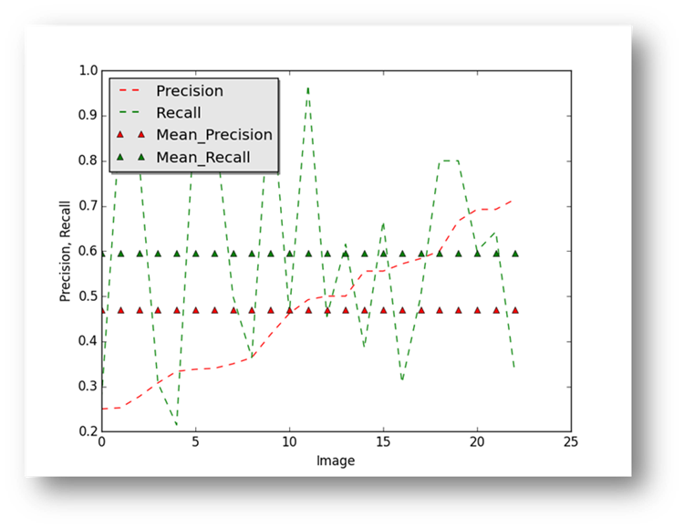
Figure24

Figure25
Figure26
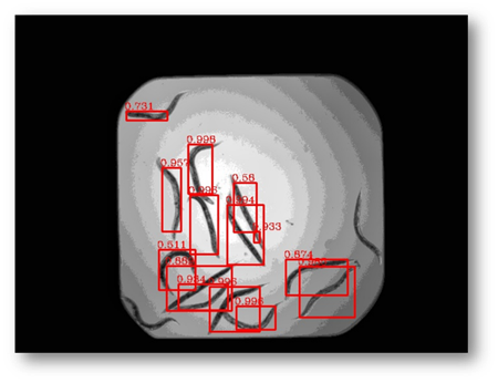
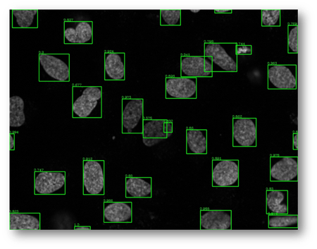
Figure27(a,b)

Figure28a
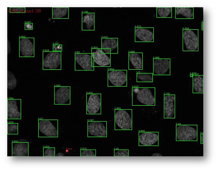
Figure28b
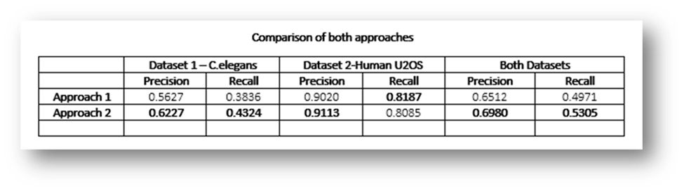
Figure29
Conclusions
Qualitative Results
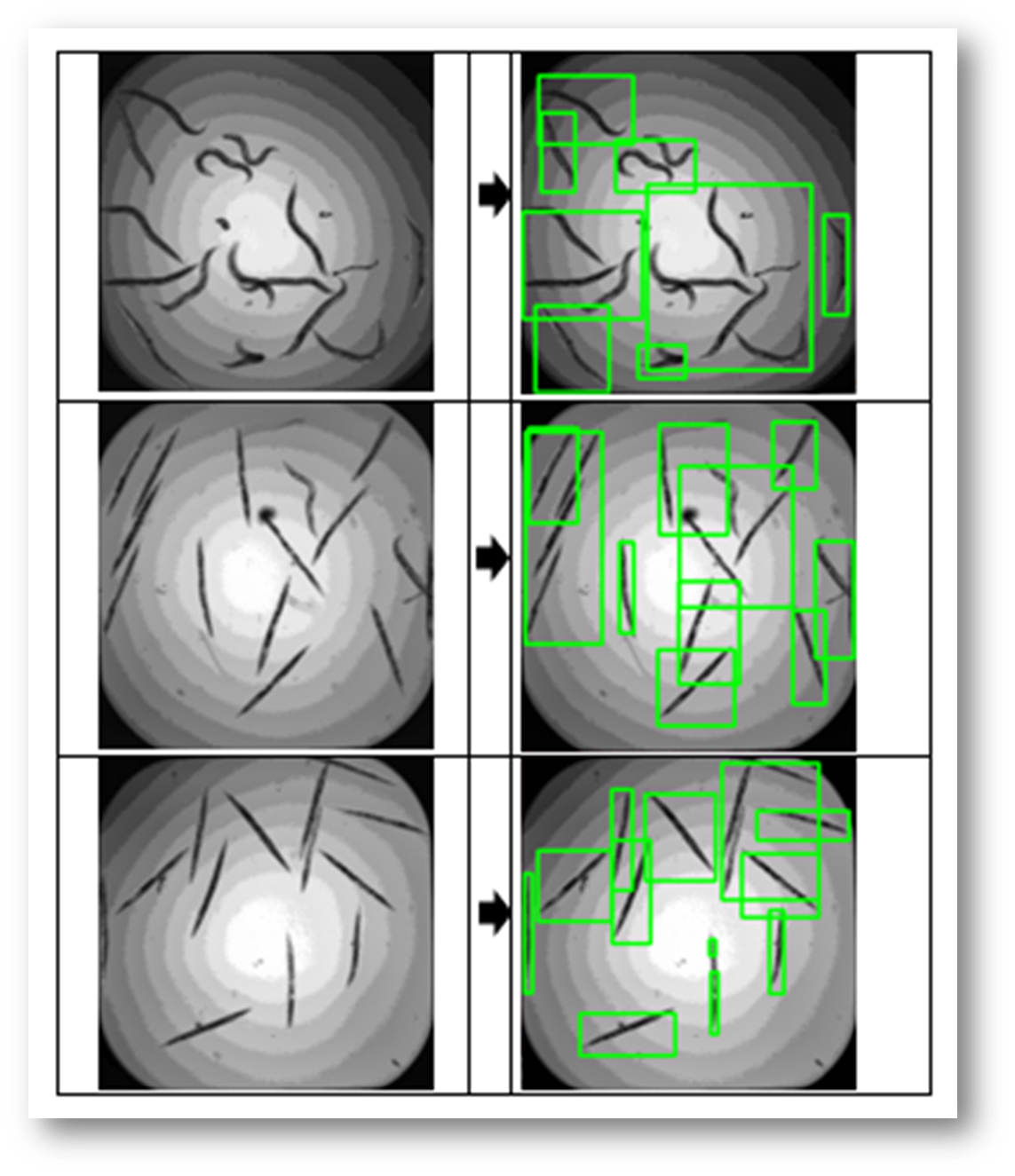
Figure30
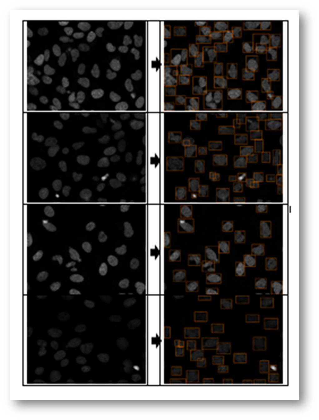
Figure31
Our Team

Swazoo Claybon
-
Divya Bala
-