%matplotlib inline
import matplotlib.pyplot as plt
import numpy as np
Caso de estudio - Clasificación de texto para detección de spam en SMS
Primero vamos a cargar los datos textuales del directorio dataset que debería estar en nuestra directorio de cuadernos. Este directorio se creó al ejecutar el script fetch_data.py desde la carpeta de nivel superior del repositorio github.
Además, aplicamos un preprocesamiento simple y dividimos el array de datos en dos partes:
text: una lista de listas, donde cada sublista representa el contenido de nuestros sms.y: etiqueta SPAM vs HAM en binario, los 1 son mensajes de spam mientras que los 0 son mensajes ham (no spam).
import os

with open(os.path.join("datasets", "smsspam", "SMSSpamCollection")) as f:
    lines = [line.strip().split("\t") for line in f.readlines()]

text = [x[1] for x in lines]
y = [int(x[0] == "spam") for x in lines]
text[:10]
y[:10]
print('Número de mensajes de ham/spam:', np.bincount(y))
type(text)
type(y)
Ahora dividimos nuestro dataset en dos partes, una de entrenamiento y otra de test:
from sklearn.model_selection import train_test_split

text_train, text_test, y_train, y_test = train_test_split(text, y,
                                                          random_state=42,
                                                          test_size=0.25,
                                                          stratify=y)
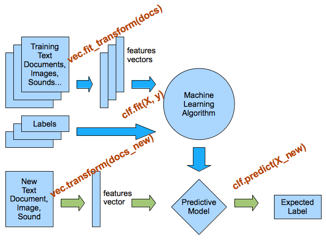
Pasamos a usar CountVectorizer para convertir el texto a un modelo bag-of-words:
from sklearn.feature_extraction.text import CountVectorizer

print('CountVectorizer parámetros por defecto')
CountVectorizer()
vectorizer = CountVectorizer()
vectorizer.fit(text_train) # Ojo, el fit se aplica sobre train

X_train = vectorizer.transform(text_train)
X_test = vectorizer.transform(text_test)
print(len(vectorizer.vocabulary_))
X_train.shape
print(vectorizer.get_feature_names()[:20])
print(vectorizer.get_feature_names()[2000:2020])
print(X_train.shape)
print(X_test.shape)
Entrenar un clasificador para texto
Ahora vamos a entrenar un clasificador, la regresión logística, que funciona muy bien como base para tareas de clasificación de textos:
from sklearn.linear_model import LogisticRegression

clf = LogisticRegression()
clf
clf.fit(X_train, y_train)
Evaluamos el rendimiento del clasificador en el conjunto de test. Vamos a utilizar la función de score por defecto, que sería el porcentaje de patrones bien clasificados:
clf.score(X_test, y_test)
También podemos calcular la puntuación en entrenamiento:
clf.score(X_train, y_train)
Visualizar las características más importantes
def visualize_coefficients(classifier, feature_names, n_top_features=25):
    # Obtener los coeficientes más importantes (negativos o positivos)
    coef = classifier.coef_.ravel()
    positive_coefficients = np.argsort(coef)[-n_top_features:]
    negative_coefficients = np.argsort(coef)[:n_top_features]
    interesting_coefficients = np.hstack([negative_coefficients, positive_coefficients])
    # representarlos
    plt.figure(figsize=(15, 5))
    colors = ["red" if c < 0 else "blue" for c in coef[interesting_coefficients]]
    plt.bar(np.arange(2 * n_top_features), coef[interesting_coefficients], color=colors)
    feature_names = np.array(feature_names)
    plt.xticks(np.arange(1, 2 * n_top_features+1), feature_names[interesting_coefficients], rotation=60, ha="right");
visualize_coefficients(clf, vectorizer.get_feature_names())

vectorizer = CountVectorizer(min_df=2)
vectorizer.fit(text_train)

X_train = vectorizer.transform(text_train)
X_test = vectorizer.transform(text_test)

clf = LogisticRegression()
clf.fit(X_train, y_train)

print(clf.score(X_train, y_train))
print(clf.score(X_test, y_test))
len(vectorizer.get_feature_names())
print(vectorizer.get_feature_names()[:20])
visualize_coefficients(clf, vectorizer.get_feature_names())

- Utiliza TfidfVectorizer en lugar de CountVectorizer. ¿Mejoran los resultados? ¿Han cambiado los coeficientes?
- Cambia los parámetros min_df y ngram_range del TfidfVectorizer y el CountVectorizer. ¿Cambian las características que se seleccionan como más importantes?