SIREN Help

All acronyms used in this help are defined in the list of acronyms
(Click the small icon on the top right of the page to return to the top)

SIREN - SEN's Interactive Renewable Energy Network tool

The SEN SAM simulation, SIREN, is used to calculate energy generation for renewable energy power stations. The program uses the SAM SDK API for energy calculations. SAM is provided by the NREL. This help briefly describes how to use the simulation.

Contents

• Licence
• Overview
• Installation
• Execution of SIREN
• Sample SIREN Model
• Setting Up
• Simulation Objects
• Stations
• Grid Lines
• Types of Grid Lines
• Preferences
• Using the Simulation
• Powermap
• Menu Structure
• Right Mouse Click
• Power Model Options
• Charts
• Tables
• Financial Model Options
• Renewable Resource Grids
• Data View
• Performance and Execution Tricks
• Powermatch
• Inputs
• Execution
• Batch
• Optimisation
• Other Charts
  • Powerplot
  • Flexiplot
• Feedback
• SIREN File Formats
• SAM Wind Turbines
• Supporting Notes
• Obtaining a Suitable Map Image
• Obtaining Current SWIS Facilities
• Obtaining and Using Satellite Reanalysis Data for SAM weather files
• Obtaining and Using ECMWF ERA5 Data for SAM weather files
• Validation of ECMWF ERA5 Data and the SAM Models
• Obtaining and Using NASA MERRA-2 Data for SAM weather files
• Validation of NASA MERRA-2 Data and the SAM Models
• Produce wind and solar weather files
• Using other Weather Files
• Visualising Renewable Resource Attributes
• SAM Models used by SIREN
• Other Models used by SIREN (experimental)
• Select area on world map
• Acronyms

Licence

Overview

Welcome to SEN's renewable energy conceptual simulation - SIREN.

The worlds renewable energy resources could provide many times the amount of fossil-fuelled energy currently used. SEN's computer simulation models an electricity network and allows you to create, cost and evaluate scenarios for supplying electricity using a mixture of renewable energy sources.

By placing virtual renewable energy plants around the area of interest, you will be able to determine the optimal locations to access renewable energy sources, minimise grid connection costs and meet the varying demand on the grid, while achieving the best in terms of efficiency, cost effectiveness and energy security.

This version of the Simulation uses the SAM SDK API for energy calculations. SAM is provided by the NREL.

Southern Western Australia (WA)

The default data provided with SIREN is for the SWIS in southern WA but the program(s) have been constructed to cover any geographic area with the appropriate input files. The techniques to create the required data files is documented in Supporting Notes.

About SEN

Our Definition of Sustainable Energy: “Energy that is renewable within a human lifetime and can be produced safely and equitably for all time with minimal impact on the environment and future inhabitants”. We believe this does not include nuclear power with its many unresolved issues.

Our Focus: To raise awareness of how a mix of renewable energy technologies are able to meet WA's energy needs, with a particular focus on the main electricity grid, the SWIS.

Our Computer Simulation (SIREN): To demonstrate how electricity demand on the SWIS may be met by a mix of renewable energy sources. Users are able to explore potential location and scale of renewable energy sources (stations, storage, transmission) to meet electricity demand.

Installation

At present there is a packaged version of the simulation for Windows available as a self-extracting zip file from https://sourceforge.net/projects/sensiren/ (the package has been created with PyInstaller). There are a number of files available:

• siren_toolkit.exe contains the full SIREN toolkit, It contains the contents of three other files in this list
• siren_application.exe contains the packaged Windows version of the SIREN application
• siren_sample.exe contains the files and data for the sample SIREN simulation of the SWIS
• (sen_makeweather_getera.exe is a package containing getera5, which enables ERA5 files to be downloaded, getmerra2, which enables MERRA-2 files to be downloaded, and makeweatherfiles, a standalone program to produce SAM weather files. This package allows you to create SAM weather files from either ERA5 or MERRA-2 files without requiring any other parts of SIREN. See makeweatherfiles.html)

Occasionally new versions of some of the SIREN programs will be uploaded to SourceForge. You can check for new versions and download them by selecting the sirenupd option in SIREN. (Major new releases can also be indicated but these will require a complete new SIREN version to be installed.)

To install the required package you can just open/launch it and extract it to your desired location. It may be necessary to execute the program as Administrator.

It is also possible to install and run the Python programs. SIREN_Notes.html provides some guidance on how to do this.

Note: This help file may refer to individual programs either with or without the program suffix, for example powermap, powermap.exe or powermap.py. You may have to use the appropriate suffix for your environment.

Possible folder setup for SIREN

To enable new versions of SIREN to be installed without affecting your work a folder structure similar to the following is suggested.

You can indicate the location of your SIREN Models in one of two ways.

1. Set up a (Desktop) Shortcut with the following Target to invoke SIREN (see below for further details):

         "C:\..Your Folder\siren\siren.exe"
   

2. Using the folder structure above as an example, set up a (Desktop) Shortcut with the following Target to invoke SIREN:

         "C:\..Your Folder\siren\siren.exe" "..\models"
   

When setting up files and folders in your Preferences file (documented in Preferences) you can use relative addresses to point to the correct location. The addresses are relative to the siren folder. For example:

      [Parents]
      $user1=../Your model
      ...
      [Files]
      solar_files=$user1/weather_files
      ...

Execution of SIREN

To execute the simulation open siren.exe in the upper folder, siren. You can easily set up a Desktop shortcut to point to the model. The package contains a number of folders with default files, some that can be replaced with your own. The location of these files are defined in a Preferences file as documented in Preferences. The default files are located in the following folders:

• siren_files contains a range of files to enable operation of the simulation
• sam-sdk contains a Windows version of the SAM SDK, sam-sdk-206_2018.11.11_r2
• source contains the Python source programs for SIREN

The first time you open SIREN (without passing a target file or folder) it will present a window titled ‘Choose location for SIREN model (preferences) files’ to allow you to choose the location for your SIREN Models. SIREN stores this location in siren_models_location.txt in a user folder and uses this as the location of the SIREN Models whenever you invoke SIREN without a target file or location. In windows the file is stored in the user's LocalAppData folder, C:\User\<user>\AppData\Local\siren\, and in Linux it is in ~/.siren/. The file contains a single line with the location of the folder respective to the siren folder. It is possible to edit the file and manually add additional folders if desired.

When you open SIREN you will be presented with a list of SIREN Models (Preferences files). Choose the SIREN Model you want by (left-) clicking on your choice to invoke Powermap for that model. It is also possible to launch tools for the model by right-clicking on your choice - the tools are as described in Tools - or you can edit the Model file. You can sort the list presented in order of either Preferences File, SIREN Model or Date modified (last time the Preferences file was saved) by right-clicking the appropriate column header. If a Model file has a syntax error this will be identified in the SIREN Model field; editing such a file will, where possible, highlight the line in error. If you want to use a specific Preferences file you can open the simulation passing the alternate filename, or a folder, as a parameter, as in these examples:

      siren.exe
      siren.exe SIREN_NWIS.ini
      siren.exe ../<folder>/SIREN_NWIS.ini
      siren.exe ../<folder with preferences files>/

If you specify a folder you will be presented with a list of SIREN Models (Preferences files) in that folder. You can either specify the folder as the full path or relative to the siren folder. Placing your models in a separate folder will make it easier to install updates to SIREN without impacting your data files.

If you want to create a new Model press the New Model button on the start up menu. You will be presented with a small list of Properties to update to create a new Preferences file. Many of these properties relate to files and file locations as described in Setting Up. It's important to ensure they're correct for the new model to open. For the file fields click on the field to navigate to the desired file or folder. At the bottom of the Create Preferences file menu you have options to Save the new file, Save the new file and edit it, or Save it and open (launch) the new model. If you specified a folder when you opened SIREN, the new model will be saved in that folder.

When you launch a SIREN model you may receive either a warning message or a status window indicating possible issues with the Preferences file (Notes in Preferences might assist).

SIREN Menu Options

SIREN has a small number of menu options.

Tools	Invoke SIREN tools. This will launch the chosen tool as a new task   flexiplot               Invoke flexiplot to create charts from Excel columns or rows (see Flexiplot)   getera5 Invoke getera5 to download ERA5 data files (see Get ERA5 Files)   getmap Invoke getmap to create a map image for SIREN (see Obtaining a Suitable Map Image)   getmerra2 Invoke getmerra2 to download MERRA-2 data files (see Get MERRA-2 Files)   makeweatherfiles Invoke makeweatherfiles to create weather files for SAM (see Produce wind and solar weather files)   powerplot Invoke powerplot to create charts from Powermodel and Powermatch outputs (see Powerplot)   sirenupd Occasionally new versions of some of the SIREN programs will be uploaded to SourceForge. You can check for new versions and download them by selecting this option
Right-click Tools	Invoke additional SIREN tools. Right-clicking on a model will present a menu of tools, as above, plus these additional tools for the chosen model   indexweather Invoke indexweather to create an index for weather files (see Using other Weather Files)   makegrid Invoke makegrid to create resource grid file (see Visualising Renewable Resource Attributes)   powermap Launch powermap for the chosen Model   powermatch Invoke powermatch to match generation to demand (load) and to quantify and cost dispatchable energy generation, storage and CO2‑e emissions (see Powermatch)   updateswis Invoke updateswis to update the list of existing SWIS Stations (facilities; see Existing Stations (Facilities)) or SWIS Load data   Edit Preferences Edit the Preferences file. This option invokes a simple text editor to allow the whole file to be edited   Edit File Preferences Edit Parents, Files and SAM Modules Sections of the Preferences file. These sections mainly have file and folder Properties. By clicking on a Property you can navigate to the desired file or folder.   Copy Preferences Copy the chosen Preferences file. This option allows you to copy an existing Preferences file - with a new name   Delete Preferences Delete the chosen Preferences file. This option allows you to delete the chosen Preferences file. A confirmation pop-up will be displayed to ensure you have chosen the correct file (theer are sometimes cases where the incorrect file may be chosen by the program so beware)
Help	Display some help about the program   Help (F1) Display the help file. The default help file, help.html, is a standard HTML file which can be displayed with your browser   About (Ctrl+I) Display details about the simulation including any licensing conditions

Sample SIREN Model

The sample SIREN model is for the SWIS for 2014 and 2015. The default Preferences files, SIREN.ini, is set up for this data and assumes the siren_sample folder is located in the same parent folder as the siren folder. The sample data contains:

• sample_files contains a range of files for the SWIS such as maps, existing network and so forth
• solar_weather contains solar (.smw) weather files for the SWIS for 2014 and 2015
• wind_weather contains wind (.srw) weather files for the SWIS for 2014 and 2015

Setting Up

The simulation uses external data files to model the potential for renewable energy generation for a geographic region. The approach is to model the data on an hourly basis for a desired year (ignoring leap days, that is, 8,760 hours). The following data files are required / desirable. Due to the initial source for each data file the format for each is different (see SIREN File Formats for further details). Please feedback any desired formats as it's relatively easy to accommodate standard file formats.

• A map of the area of interest (identified in the [Map] Section of the Preferences file). A simple JPEG or PNG image is fine although most conventional image formats should be acceptable. The map covers a geographically “rectangular” area of the earth. Obtaining a suitable map image is described in Obtaining a Suitable Map Image
• Names and locations of towns. Two files are used as input (either or both can be specified):
  1. Either a CSV or Excel (XLS or XLSX) file containing a list of weather stations from the BOM (identified by bom property of the [Files] Section of the Preferences file)
  2. Either a CSV or Excel (XLS or XLSX) file containing the location of additional towns or localities (identified by towns property of the [Files] Section of the Preferences file)
• Names, technologies and locations of existing power stations (identified by grid_stations property of the [Files] Section of the Preferences file). This is either a CSV or Excel (XLS or XLSX) file which contains details of existing Facilities (Stations) registered with the local electricity regulator (AEMO in the case of the SWIS) augmented by geographic location of the station and details on turbines for wind farms. The CSV file may be either a specific format or a normal scenario file. You can update this file for the SWIS as described in Obtaining Current SWIS Facilities.
  You can also create additional stations, such as Rooftop PV, to be included in the list of existing stations by creating an additional Stations file and setting the grid_stations2 property in the [Files] Section of the Preferences file
• A layout of the existing electrical grid. A KML file showing the layout of the major power lines in the grid and another with the outline of the network (SWIS) boundary. This should be a simplified version of the grid network with all lines connecting exactly for SIREN to correctly connect new stations into the grid
  Note: The intention of these two files is to describe the existing fossil and renewable Stations on the electricity network
• Optionally, the network can be divided into zones. This enables different renewable energy potential between zones to be analysed and utilised by Powermatch
• Hourly load details for the electricity grid. Either a CSV or Excel (XLS or XLSX) file with a single column of electrical load data for the 8,760 hours in the year of interest (identified by load property of the [Files] Section of the Preferences file). Each value is for one hour of load commencing on that hour.
• Hourly solar and weather details for the area of interest (identified by solar_files and wind_files properties of the [Files] Section of the Preferences file). This data is in formats required for input to SAM and contains entries for the 8,760 hours in the year of interest. A SAM weather file is a text file that contains one (calendar) year's worth of data describing the solar resource, wind speed, temperature, and other weather characteristics at a particular location. The approach we have adopted is to use satellite data, either ECMWF ERA5 data or NASA MERRA-2 data, for the desired geographic area and year to create appropriately formatted weather files. This is described in Obtaining and Using ECMWF ERA5 Data for SAM weather files. To enable more recent (part-year) data to be used it is possible to “wrap” the data by using the weather data for the prior year for the remaining part of the year.
  You can also use TMY files such as those provided with SAM. If you have a number of weather files you can create an index of these files for SIREN. This is described in Using other Weather Files
• SIREN allows you to visualise renewable resource attributes. This utilises a summary file to avoid having to process all the weather files covered by the map (identified by resource_grid property of the [Files] Section of the Preferences file). This is described in Visualising Renewable Resource Attributes

You can successfully use the simulation with just the map and weather data while existing load and network data enhance it's usefulness.

A note about hours

Due to inconsistency between power (SAM) and weather data / files, hours of the day are portrayed differently. For example, looking at the hour between midnight and 1:00AM:- in power data the hour is shown as the start of the hour, 00:00, while for weather data it is the end of the hour, 01:00.

Simulation Objects

The simulation has two main objects, stations and grid lines. Stations can be saved as scenarios in either an Excel (XLS or XLSX) or CSV file format while grid lines are constructed during the simulation rather than being saved to a file (unless you have manually created the grid line).

Stations

Stations represent either existing generation stations on the grid or new ones you have created during a simulation session. The station files can be updated outside of the simulation. The fields for a station are:

When you display a Station with SIREN it will also show the Scenario the Station is in. For new Stations (i.e. not Existing) it is possible to update this value to one of the other scenarios that are currently “open“. This will move the Station into that scenario and, if the scenario is saved move it permanently into that Scenario.

Grid Lines

Grid lines connect new stations to either existing or other new grid lines. By default the grid line will connect a station to the nearest point on the grid. You can edit a grid line if you wish to connect it elsewhere in the grid. Grid lines are recalculated when you add or modify stations but are not normally saved. You can, however, list the (new) grid lines and save the table listed. The fields for a grid are:

Types of Grid Lines

A grid is built up of a number of different types of line to enable differing loads to be carried. Each line has a maximum carrying capacity. Greater loads require additional lines to be added; so in this simulation one line may represent multiple grid lines as described in the Line Table for the line. For dispatchable transmission we need an extra path for backup purposes (N-1) while no such backup is required for non-dispatchable loads (N-0). For a line carrying both we'll use a criteria of N-0 for total load plus N-1 for dispatchable load. Within this simulation line types and costs can be specified (somewhat cryptically) in the [Grid] Section of the Preferences file. The default set of lines are:

Above 500MW it's a case of alternately adding 330_s and 330_d costs.

Preferences

Many options can be specified by a Preferences file. When you open SIREN you will be presented with a list of available Preferences files (SIREN Models) to choose from. These files reside in the same folder as SIREN itself (they may be placed in a different folder by passing that folder as a parameter when SIREN is invoked). The format is similar to a Windows INI file. If you want to create a new Model you can press the New Model button on the start up menu. You will be presented with a small list of Properties to update to create a new Preferences file.

The Preferences file has the following Sections and properties. The file is a simple text file which must be saved in the siren folder and have a file type of .ini (INI File). The sample siren_default.ini or siren_windows_default.ini file will provide a useful guide as to the content.

There are three special strings which will be replaced in the Files properties variables:

• $USER$ will be replaced with the current userid
• $YEAR$ will be replaced with the base year value
• $dirn will be replaced with the corresponding variable from the [Parents] Section

Note: Technologies appear in two forms in the Preferences file. They appear in the Preferences Sections as words starting with an uppercase letter and separated by spaces (e.g Fixed PV with the Section name [Fixed PV]). In the Section Properties the technology names are changed to all lower case and spaces are replaced by underscores. Thus, Fixed PV will appear as fixed_pv. The lower case versions occur in the [Colors] Section and [Grid] dispatchable, [Power] fossil_technologies, and [Power] technologies variables.

(Skip to Using the Simulation)

Shortcut to Sections:- Backtrack PV, Base, BESS (Battery), Biomass, Colors, CST, Dataview, Dual Axis PV, Files, Financial, Fixed PV, Flexiplot, Fossil Coal, Fossil Cogen, Fossil Gas, Fossil Mixed, Geothermal, Grid, Hydro, Map, Offshore Wind, Other, Parents, Plot Colours, Power, Powermatch, Powerplot, PV, Rooftop PV, SAM Modules, Single Axis PV, Solar Thermal, Storage, View, Wave, Wind, Windows.

Using the Simulation

The SIREN simulation has two parts:

1. Using Powermap to build scenarios for an energy mix and calculating the renewable energy produced. It allows you to “map” renewable energy generation. This is described in Powermap
2. Using the Powermatch data produced by Powermap to complete a costed renewable energy scenario. It allows you to “match” renewable energy generation to demand. This is described in Powermatch

There are also a few other programs that augment the results and data produced by Powermap and Powermatch.

Powermap

Powermap allows you to build scenarios for the energy mix for your area of interest. It is based around the map of your chosen area and allows you to visualise the layout of the existing electricity network plus the additional stations you place on the map to build your scenario(s). The map initially shows the main skeleton of the existing electricity grid infrastructure and current generation stations.

To add a new station simply right-click on the map at the desired location and then update the details for the station (Name, Technology, Capacity and so forth) and press Save & Exit. You can also copy an existing station and other options as specified above.

As you build your scenario, the simulation adds additional infrastructure to connect the new generation plants to the grid. The colours for the majority of the items on the map are as you specify in the Preferences file. You navigate around the map using normal mouse movements to scroll, zoom, etc. and interact with it as described in Menus. Using the various menu options you can model your whole scenario, or by right-clicking you can deal with an individual station. There are a number of additional windows, such as menu options, that can be opened to assist with using Powermap (see Windows)

You can save multiple scenarios and add them and remove them as you wish. When you exit the simulation normally or Save scenarios (Ctrl+S) any modified scenarios will be saved. When you add new stations to your model they will be added as a new scenario which includes the date and time in its name, for example, Scenario_2015-06-09_1000. You can save all open scenarios as a single new scenario by using the Save As... option.

The strength of the simulation is in running the SAM Power Models (e.g. Ctrl+P). This will run the appropriate SAM model for each station you have chosen or for all renewable stations in your current simulation. SAM calculates a list of power outputs for each hour of the year (8,760 points). If the show_menu property is True you will be presented with a menu to specify what processing and charts to produce (see Power Model Options below). If you choose to run the Financial Models or Powermatch you will be presented with an additional menu of options.

• The various charting features allow you to visualise the renewable energy output and how it compares to demand
• The Financial Models option will invoke SAM Annual Output and Utility IPP/Commercial PPA Finance models. These enable a LCOE to be determined for the scenario
• Powermatch allows you to complete a costed renewable energy scenario. It will use dispatchable generation to meet shortfalls in the renewable energy generation mix to match generation with demand (load) to quantify and cost dispatchable energy generation, storage and CO₂‑e emissions

Usage Notes:

• To simplify the inputs required to run the SAM Power Models Powermap uses variable files for most of the input variables as described in SAM Models used by SIREN. You can change the default inputs by editing or creating your own copy of the variable files. With the One variable you may want to adjust is the hub height in the windpower model
• If you run a simulation and get generation of 0 for a station it may be because SAM has returned an error; the error message will appear in the Status Window. If you don't normally have the Status Window open you can Open the window via the Powermap Windows sub-menu and rerun the Power models to find the error

Notes on Wind Stations

With increasing hub heights associated with larger turbines the SAM models are impacted by the lack of suitable wind speed data at greater heights. The MERRA-2 climate data has a maximum wind speed height of 50 metres which will cope with hub heights up to 85 metres (above that height the SAM windpower model will fail with an error - “... the closest wind speed measurement height (50 m) found is more than 35 m from the hub height specified”). To overcome the wind data limitation Powermap can extrapolate wind speeds to greater heights. To enable this you can use the hub_formula property of the [Wind] and [Offshore Wind] Sections of the Preferences file (behaviour can also be changed with the hub_spread property). This formula can be used to calculate a hub height (for rotor lengths greater than 85) and to extrapolate wind speed using either of two commonly used laws (models). The law to be used can be specified in the extrapolate property of the appropriate wind Section(s) and can be either logarithmic, the default, or Hellmann. This additional data will be added to the normal wind file and passed to the SAM windpower model. If you wish to use this you need update the windpower variables file to allow the default hub height (85 m) to be overridden.

From ‘Do we really need rotor equivalent wind speed?’ (Van Sark etal, https://onlinelibrary.wiley.com/doi/full/10.1002/we.2319#:~:text=For%20situations%20where%20the%20ratio,and%20the%20wind%20speed%20at) a possible formula for calculating hub height is - H = 0.789 D + 14.9 m. For the hub_formula property this can be set as:

hub_formula=int(floor((0.789 * rotor + 14.9) / 5) * 5)

Powermap will replace rotor with the rotor diameter for the station turbine and perform the calculation which will round the calculated hub height down to the nearest 5 metres. You can of course just set hub_formula=90 to set a fixed height

Discussions on the two wind profile laws can be found at Wind profile power law (aka Hellmann law) and Log wind profile (aka logarithmic law). The Hellmann law tends to give slightly higher wind speeds. ‘Methodologies Used in the Extrapolation of Wind Speed Data at Different Heights and Its Impact in the Wind Energy Resource Assessment in a Region’ (https://www.researchgate.net/publication/221912731_Methodologies_Used_in_the_Extrapolation_of_Wind_Speed_Data_at_Different_Heights_and_Its_Impact_in_the_Wind_Energy_Resource_Assessment_in_a_Region) provides a fuller discussion on the topic.

Menu Structure

The Powermap menus allow you to interact with the full simulation while right-clicking the mouse allows you to interact at the detail of an individual station. The majority of the menu options have a keyboard shortcut. The layout of the menus are set out below (Note: Sometimes the menu options will disappear from the menu bar. The easiest solution is to maximise the main window and then restore it to it's normal size)

Scenario	Work with scenarios. It is possible to edit the scenarios outside of the simulation as they are simple CSV or Excel (XLS or XLSX) files. The type of file is indicated by the file type - .csv for a CSV file, or .xls or .xlsx for an Excel file. If the file type isn't specified any scenario will be saved in Excel (XLSX) format.   Open (Ctrl+O) Open an existing scenario. This will open the selected scenario and replace all stations in the current session with those in the chosen scenario   Add (Ctrl+A) Add all the stations from an existing scenario to the current session   Remove           ...Scenario(s) Remove one of the open scenarios stations from the current model. The Existing scenario allows you to remove existing stations from your session   Edit Descr.           ...Scenario(s) Edit the description for a scenario in the current model   Save (Ctrl+S) Save any scenarios modified in the current model   Save + Desc Save any scenarios modified in the current model and allow descriptions to be updated   Save As... Save the current model as a new scenario   Exit (Ctrl+X) Save any modified scenarios and exit the simulation   Quit (Ctrl+Q) Quit the simulation without saving any changes   Add Existing If you have removed Existing Stations this option will allow you to add them back
Power	Run SAM models for the current model or list details on new infrastructure in the model   Power for yyyy (Ctrl+P) Run SAM models for the base year for each station in the current model and display power curves for the full model   Power for year           ...years(s) Run the SAM Power Models for one of the years available   List Stations (Ctrl+L) List stations in the current model. This will list either all renewable stations or, if 'Display fossil-fuelled stations' is set, all stations including fossil-fuelled stations. By right-clicking a column header you can sort by that column in ascending and then descending order. By left or right-clicking a station you can display the details for that station   List Grid (Wires; Ctrl+W) List grid network lines in the current model. By right-clicking a column header you can sort by that column in ascending and then descending order. If [Grid] trace_existing is set existing grid lines will also be displayed   Save Stations (as KML) Save the current stations as a KML file which can be displayed in Google Earth. The stations will display as a small pin; hovering over a station will display it's name   Save Grid (as KML) Save the current grid as a KML file which can be displayed in Google Earth   Load for yyyy Display load curves for the base year. An options menu is displayed to enable you to choose which charts you want. The options are as described in Choose charts in Power Model Options.   Load for year           ...years(s) Display load curves for one of the years available ...   SAM Version Display the version of the SAM SDK used by this model ([Files] sam_sdk property). Details will be shown in the status line at the bottom of the main window   Exit Visualise This will allow you to exit visualisation of generation
View	Modify the view of certain elements of the simulation. Those identified with a tick icon can be toggled on or off   Show Capacity Circles (Ctrl+C) Display circles for the stations based upon Capacity (True) or station area (False)   Show Generation Circles (Ctrl+K) Display circles for the stations based upon Generation (True). This will only display circles for stations that have had the Power model run for them   Show Station Names (Ctrl+N) Display all station names (True) or just the current one (False)   Show Fossil-fuelled Stations (Ctrl+F) Display fossil-fuelled stations (True)   Show Scale Ruler (Ctrl+R) If True Display a Scale Ruler. If you want to move the ruler you need to toggle it off and then back on again   Show Legend If True Display a legend. The legend displays coloured circles for each technology on the map and squares indicating the total land area occupied by these technologies. The legend will be placed (top) right of the map   Show Towns Display Towns (True)   Show Existing Grid (Ctrl+H) Display the existing grid network (True)   Show Existing Grid2 (Ctrl+2) Display the existing detailed grid network if one is available (this grid is not utilised by Powermap; True)   Show Grid Zones Display grid zones if available   Show Station Connections Display transmission lines that connect stations into the grid   Clear Grid Trace Clear any grid trace   Show Grid Line (Ctrl+J) The option allows you to choose an existing grid line to trace it's path   Refresh Grid This is a temporary option to refresh the Grid if the grid tracing and shortest path algorithms misbehave   Show Coordinates Grid Display a grid of latitude and longitude. The spacing of the grid is based upon the geographic size of the map.   Show Grid Areas Display grid areas if available   Go to Station (Ctrl+G) Centre the view on a particular station selected from a list   Go to Town (Ctrl+T) Centre the view on a particular town selected from a list   Go to Location (Ctrl+D) Centre the view on a particular location   Go to Load Centre (Ctrl+M) Centre the view on a Load Centre   Save View (Ctrl+V) Save the current view to an image file
Preferences	Edit or display aspects of the Preferences file. Changes for some variables will take effect immediately on exit from the edit program while others (such as the map) will require you to restart the simulation   Edit Preferences File(Ctrl+E) Edit the Preferences file, either SIREN.ini or that file passed as a parameter when you invoked the simulation. This option invokes a simple text editor to allow the whole file to be edited   Edit Colours (Ctrl+U) Edit colours for the current map. This will allow to change both the colours for the current map_choice (left column) and the default colours (right column). You can delete colours for the current map_choice by right-clicking on the colour (it will be cleared and the item deleted when you Save & Exit)   Edit File Sections Edit Parents, Files and SAM Modules Sections of the Preferences file. These sections mainly have file and folder Properties. By clicking on a Property you can navigate to the desired file or folder.   Edit Section Edit a specific Section of the Preferences file. You will be presented with a list of Sections to choose the desired one. The edit program will then present a table of current Properties and their values. It is also possible to add values for Properties not currently present in that Section   Edit Technologies Edit standard Properties for all Technologies. This option allows you to edit the “standard” variables for all technologies (area, capital_cost and o_m_cost)   Dispatchable Lines Table This will list the dispatchable_lines table showing the range of dispatchable lines for each level of peak dispatchable capacity   Standard Lines Table This will list the standard_lines table showing the range of standard lines for each level of peak capacity   Line Costs List the cost per km for each type of line   Substation Costs List the substation cost for each type of line
Windows	Display additional (floating) windows. These windows can be opened and still allow interaction with the main Powermap window. if restorewindows is set Powermap will remember the placement of windows and restore them as closely as possible to these positions when they are next opened.   Credits (F2) Display Credits window - brief details about SIREN, acknowledgements and licensing   Show Resource Grid (Ctrl+B) Invoke Resource Grid window to display gridded resource data on the map   Resource for year           ...years(s) Invoke Resource Grid window for one of the years available   Show Floating Legend Invoke Floating Legend to display a legend in a floating window   Show Floating Menu Invoke Floating menu window to display Powermap menu options   Show Status Window Invoke floating window to display a log of Powermap session activity and open scenarios   Show Data View Invoke Data View window to display “gridded” contribution to generation on the map
Tools	Invoke SIREN tools. This will launch the chosen tool as a new task   getera5 Invoke getera5 to download ERA5 data files (see Get ERA5 Files)   getmap Invoke getmap to create a map image for Powermap (see Obtaining a Suitable Map Image)   getmerra2 Invoke getmerra2 to download MERRA-2 data files (see Get MERRA-2 Files)   indexweather Invoke indexweather to create an index for weather files (see Using other Weather Files)   makegrid Invoke makegrid to create resource grid file (see Visualising Renewable Resource Attributes)   makeweatherfiles Invoke makeweatherfiles to create weather files for SAM (see Produce wind and solar weather files)   powermatch Invoke powermatch to match generation to demand (load) and to quantify and cost dispatchable energy generation, storage and CO2‑e emissions (see Powermatch)   powerplot Invoke powerplot to create charts from Powermodel and Powermatch outputs (see Powerplot)   updateswis Invoke updateswis to update the list of existing SWIS Stations (facilities; see Existing Stations (Facilities)) or SWIS Load data
Help	Display some help about the program   Help (F1) Display the help file. The default help file, help.html, is a standard HTML file which can be displayed with your browser   About (Ctrl+I) Display details about the simulation including any licensing conditions

Right Mouse Click

Clicking the right mouse button allows various actions for the nearest station. Dependent on the nearest station some options will not be available. The full list is as follows:

Run SAM Model	Run SAM Power Model for nearest station
Model Power for year           ...years(s)	Run the SAM Power Model for nearest station for one of the years available
Copy station	Copy nearest station. After selecting this option and updating any changed details move the mouse to the new location and press the left mouse button to locate the new station
Centre view	Centre view on nearest station
Show/Edit details	Show details for nearest station. If it is a new (i.e. not an existing) station you can also edit the stations details
Move	Move nearest station. After selecting this option move the mouse to the new location and press the left mouse button to relocate the station
Delete	Delete nearest station
Edit grid line for station	Edit Grid line for station at (this) location. This option allows you to override the default process of connecting the grid line to the nearest existing grid line. By clicking the left mouse button you can indicate where you want the grid line to be positioned; each click adds a new leg to the grid line; double-clicking terminates the edit and connects the grid to the (now) nearest grid line
Trace grid for station	Trace Grid for station at (this) location. This option will trace the grid connection between the station and the (nearest) load centre
Add station	Add station at (this) location
Show details for nearest grid line	The nearest grid line will be highlighted and some details displayed in the Status line. Details will include the line name, length, an indication if it carries Dispatchable generation, and the peak load on the line
Show Zone for here	Display the zone for the chosen location
Show weather for here	Present a menu to allow you to chart weather values (DHI, DNI, GHI, temperature, wind speed) for this location. You select the weather values you want to display and one of a series of charts to display either by hour or the average for a period. There is also an option to display chosen charts one at a time or all together, that is, display them all and allow you to navigate between them
Weather for year           ...years(s)	Show weather here for one of the years available
Show details	Show details for nearest town
Position ruler here	Position ruler here. Position will be approximate
Position legend here	Position legend here. Position will be approximate

Power Model Options

The Power Model options menu are as set out here. The default values are specified in the [Power] Section of the Preferences file. The associated property is indicated in brackets at the end of the description. If you hover over the window title bar or press F1 a help for the Options will be displayed.

The charts and tables are intended to assist with analysing the chosen scenario.

Charts

• Save chart data will enable most of the data inputs to charts to be saved to a spreadsheet. These values are usually an aggregation of the hourly outputs produced by Power Model
  Note: If you choose the Power by hour - augmented you can estimate how much non-renewable generation is required to meet the Load (see Augmented (non-renewable) Generation)
• Visualise generation - period & delay (secs) will visualise generation by displaying variable generation circles for each station over the chosen periods. This option displays an additional window to control the visualisation:

  Detail	The choices are: Diurnal. Visualise average generation for each hour over the year (24 periods) Monthly. Visualise average generation for each hour for each month (12 x 24 periods) Hourly. Visualise generation for each hour of the year (8,760 hours)
  Period	This row provides pull-down menus to allow you to choose a period, day and hour to visualise
  <          >	You can also navigate to a particular time period by dragging the slider bar. Clicking < will step back one period while > steps forward one period. You can also use Page Down and Page Up to step forward and back
  Save Views	If the save_view property of the [Power] section is True you will be able to save individual views of the visualised generation. When you first set an increment value you will be presented with an option to specify a location for the saved files. The files will be saved in the chsoen location with a filename equal to the chosen value plus an indication of the period it relates to. This will enable you to create a video of the sequence using an appropriate tool. You set the total number of files (views) to be saved and each iteration of the visualisation will save a file and decrement the counter until it reaches zero
  Repeat Loop	If checked this option will cause the visualisation to repeat continuously
  Period Loop (secs)	You can also cause the visualisation to automatically loop through all time periods. The number field allows you to specify the delay in seconds between each period - between 0 and 10 in .2 second increments. You press the Loop button to start the loop. Press Stop (or the Power -> Exit Visualise, Ctrl+Z, menu option) to stop the loop.
  Quit	Exit the visualisation

• Energy by ... options produce step charts that aggregate data into the chosen period
• Power by hour option produce line charts for each hour of the year
• Power - diurnal ... options produce line charts that summarise data to produce an average diurnal (daily) chart for each of the chosen periods
• Power - Load duration option produces load duration curves which show how much generation is produced for a percentage of the year
• Power - Shortfall analysis option produces a table and line charts that attempt to assist with analysing shortfalls on a daily basis. The analysis iterations option will produce average shortfalls for that number of days, for example, 3 iterations will produce average shortfall figures for one, two and three days. The figures are calculated by “averaging” the generation shortfall over the chosen number of days. This option will also produce cumulative shortfall charts that add the average hourly shortfall to generation to attempt to flatten out the shortfall over the year

Refer to Other Charts for details about Plot Navigation.

Tables

• Save Hourly Data Output option will save generation in MWh for each chosen station for each hour of the year (8,760 hours) as calculated by SAM. This can be used in detailed analysis or as an option to avoid having to reprocess the station in the future, by updating a Station's Power File field. The default filename can be set using the data_file property of the [Files] Section of the Preferences file; otherwise it will in the format of Power_Table_yyyy-mm-dd_hhmm...
• Save (adjusted) Hourly Data Output by Station option will save generation in MWh for each station and other options for each hour of the year (8,760 hours). This is the hourly output calculated by the SAM model multiplied by any adjustments. If appropriate Power Model options are chosen data for Generation, Excess, Load and Storage will also be saved. The default filename can be set using the data_file property of the [Files] Section of the Preferences file; otherwise it will in the format of Power_Detail_yyyy-mm-dd_hhmm...
• Save (adjusted) Hourly Data Output by Technology option will save generation in MWh for each technology and other options for each hour of the year (8,760 hours). This is the hourly output calculated by the SAM model multiplied by any adjustments. If appropriate Power Model options are chosen data for Generation, Excess, Load and Storage will also be saved. The default filename can be set using the data_file property of the [Files] Section of the Preferences file; otherwise it will in the format of Power_Detail_Technology_yyyy-mm-dd_hhmm...
• Save Powermatch data option will save save the input data for Powermatch (or Powerbalance). There are two possible output formats:
  1. Powermatch uses scenario worksheets. If the pm_template property of the [Files] Section is set, Powermap will save the inputs in this format. The file can (only) be saved as an .xlsx format file
  2. The original Powerbalance uses the hourly shortfalls and overall generation figures in its computations. This option saves this data in a spreadsheet to simplify copying it into a Powerbalance workbook. The cells required for Powerbalance are highlighted in colour. The worksheet contains the generation summary data followed by the shortfall data. The file can be saved as .csv for a CSV file or .xls for an Excel file
• Show Summary/Other Tables option will cause various tables to be presented:
  • A brief summary table of Capacity and Output for each selected station. The default filename will in the format of powermodel_Table_yyyy-mm-dd_hhmm
  • If Storage values are specified a storage table is produced showing hourly figures for Load, Generation, Storage Used, Storage Losses (determined by Discharge and Recharge loss percentages), Storage Balance, Shortfall and Excess. Shortfall indicates the shortfall against Load (Load less Generation, Storage Used and Losses); Excess indicates excess generation that could not be stored due to either the Storage Capacity limit or Recharge cap. The default filename will in the format of Storage_Table_yyyy-mm-dd_hhmm
  • Generation Summary table is a brief summary of the overall generation for the current execution of the Power model. The figures are summations of the 8,760 hourly figures. Some comments on the table:
    • The Multiplier column indicates any multipliers from the adjust generation option (plus load if load is grown)
    • The Row column is merely a technique to display the rows in a suitable order
    • The initial rows are the totals for each of the technologies, followed by the total of all generation and the load to be met
    • Gen. - Load is a raw indicator of generation versus load but ignoring any timing issues. A negative value indicates a shortfall in overall generation while a positive value indicates excess overall generation
    • Storage Capacity is the amount of storage in this execution
    • Storage Used is how much storage has been used to meet shortfall in generation for any period. This is that portion of renewable generation that has been stored and then reused
    • Excess Gen. is energy generation that has been lost/dumped due to either full storage or constraints on storage recharge
    • Shortfall is the lack of available energy (generation plus storage) to meet load
• The Power - Shortfall analysis Plot option produces a table showing hourly figures for Load, Generation, Shortfall, and, optionally, grid losses. If iterations are chosen an additional table showing daily shortfalls for each iteration will also be produced. The default file(s) name will in the format of Hourly Shortfall_Table_yyyy-mm-dd_hhmm and Daily Shortfall_Table_yyyy-mm-dd_hhmm

Financial Model Options

Note: Implementation of the SAM Financial models in SIREN is a work in progress. If you have suggestions on how you would like SIREN to be extended in this area contact siren@sen.asn.au.

If you have chosen to run the Financial models you will be presented with an additional options menu as set out here. The default values are specified in the [Financial] Section of the Preferences file. The associated property is indicated in brackets at the end of the description. If you hover over the window title bar or press F1 a help for the Options will be displayed.

Notes on the Financial Model Table

• The table presents LCOE figures for each station and an overall LCOE estimate. The overall estimate is calculated by multiplying the LCOE for each station by the ratio of it's generation to total generation
• Strictly speaking LCOE does not include grid costs. The grid options are provided to enable the impact of this cost to be included in the model
• As mentioned previously, Include full grid path in LCOE? may over-inflate grid costs as each station path to the load centre is traced individually

Resource Grids

To assist with placement of renewable energy stations Powermap can display a grid of renewable resource attributes derived from the SAM weather files. The grid can be displayed by invoking the Show Resource Grid (Ctrl+B) menu option. The Resource Overlay menu presented has the following fields:

Altering any field will cause the revised grid to be overlaid on the Powermap map. The buttons are:

• Quit. Close the Resource Overlay menu. Any grid will continue to be displayed
• Show. Cause the grid to be displayed. This allows you to display the grid without changing any of the fields
• Hide. Hide the resource grid
• Save. Save modified fields. This updates the Preferences file for future executions of Powermap
• Help. Display the help for how to create the Resource grids
• < and >. (see above)
• Loop. (see Period Loop (secs) above)

This feature utilises summary data stored in a file rather than having to process hourly data from the weather files (see Visualising Renewable Resource Attributes).

Performance and Execution Tricks

Processing a simulation with a large number of stations can take a while to process, especially with Solar Thermal stations. You can minimise this processing by using either of these two options:

1. When you invoke Power Model processing it allows you to process Chart (and Table) options multiple times without reprocessing the stations. You can then process Financial options multiple times. The process Powermap uses is as follows:
   1. Displays the Power Model menu allowing you to specify initial options. This allows you to choose the stations of interest and the data options you want. This first display of the menu also allows you to save these options
   2. Calls the appropriate SAM module for each chosen station, or other options as specified
   3. Presents the tables and charts you have selected
   4. Re-displays the Power Model menu allowing you to specify different growth options, storage options and charts. A number of options, such as Generation - from chosen stations will no longer be available as they would require reprocessing the SAM models. To process these new options press the Proceed button. To exit this phase of processing press the All Done or Do Financials button
   5. If you have chosen to run the Financial Models the Financial Model menu will be displayed, allowing you to specify initial finance options. Press the Proceed button to continue with these options
   6. Calls the SAM financial module for each chosen station
   7. Presents the financial table
   8. Re displays the Financial Model menu allowing you to specify different options. Press the Proceed button to invoke these new options. To exit this phase of processing press the All Done button

2. If the location and size of stations haven't changed you can avoid reprocessing stations by used Power data from a previous simulation run, using the following approach.
   1. Choose the Save Hourly Data Output (save_data) Power Model option
   2. Save the data file. This file contains power output for all stations in the current simulation. It should be located in the same folder as your scenario files (scenarios property of the [Files] Section). The data is saved as MWh with 4 decimal places because SAM uses kWh
   3. With your spreadsheet application (Excel) update the scenarios and stations that you want to use the saved data with. Either add or use the column headed Power File to specify the filename you've selected for the power output. For each station enter the full name and extension of the file, for example, Power_Table_Saved.xlsx
   4. When you next run the simulation it will load this saved data rather than invoking the SAM module for each station that has an Power File entry
   5. If the file is not found the SAM module will be re-invoked. So you can simply delete or rename the Power data file and re-run the simulation to get a new set of data points

Adjust Generation

The Generation - adjust generation option allows you to easily adjust the contribution of each technology to the overall model by allowing you to apply a multiplier to the generation figures. The multiplier multiplies each hourly generation figure to approximate increasing the station by this size. This enables you to assess changes to the technology mix without having to alter individual stations. If you also choose the Generation - from chosen stations option you can also do this adjustment for each station rather than each technology. This approach allows you to “experiment” with the generation mix without having to add or alter stations.

Augmented (non-renewable) Generation

You can roughly estimate how much augmented (non-renewable) generation is required to meet the Load by selecting some appropriate Power Model options. This approach will indicate how much hourly demand can be met by generation, with or without storage, in the same hour, and how much excess renewable generation is spilled. If you choose the Save chart data and Power by hour - augmented option three tables will be produced. The first is actual data as in the graph, the second will adjust values to indicate the amount of generation from each component, and the third is a summary of the totals for the second table. This final table summarises how much demand is met by renewables and storage, how much has to be met from other sources (Augment) and how much renewable generation is spilled (that is, not used to meet demand or add to storage). This gives a slightly more accurate figure on how well your scenario meets hourly Load.

Saving the Current View

It is possible to save the current view of the main Powermap window using the Save View (Ctrl+V) option. Depending on the options chosen you can choose to crop the view at the map boundary (crop_save=True) or to save the full view, and to save either the underlying map (scene_save=True) or the screen view. The image resolution can be different in the two options, dependent upon screen resolution, image resolution, screen window size and how much of the map is being saved.

Powermatch

Running the SIREN models will produce hourly generation figures which identify generation shortfalls and excesses against load (demand). One of the outputs from Powermap is a table of these generation shortfalls which could be met by storage (charged by surplus renewable generation) and dispatchable energy generation. The Powermatch (powermatch) component of SIREN can be used to match generation with demand (load) to quantify and cost this dispatchable energy generation, storage and CO₂-e emissions. This enables you to complete a costed renewable energy scenario. If the input data spreadsheet has zones (of generation) the calculations will be performed for each zone.

A Note on Load. Load is a measure of demand on the electicity network. It can be grouped into two broad areas:

• Operational Load, or simply Load, is the demand needed to be met by the (utility-scale) generators and storage on the network. This is the load that Powermatch meets using the proposed generators
• Underlying Load is Operational Load plus additional demand that is met by “behind the meter” generation such as Rooftop PV. Powermatch adds this generation both to generation by the network and generation to meet load. Thus, these generators have no shortfall or surplus
  Identification of underlying generation is via the underlying property of the [Powermatch] Section of the Preferences file. It is also possible to indicate a specific generator is operational rather than underlying via the operational property

One of the outputs from Powermatch is calculated Levelised Cost figures for each Generator, LCOG, and Storage, LCOS, and an overall LCOE. The Levelised Costs are calculated based upon either Capital (Capex), Operations (Opex) and fuel costs or a Reference LCOE and Reference Capacity Factor (CF) for the generator or storage. Be aware that if a facility is not used it will have no costs associated with it (this is based upon the premise that the facility would not be included in any detailed modelling). Powermatch has three interpretations of levelised cost:

1. LCOG and LCOS. This is the average cost of all generation (or, in the case of storage, discharge) produced by a facility
2. LCOE. The average cost of electricity. This is generally higher as it excludes surplus - spilled or curtailed - generation from renewable technologies not used “to meet load”. This is the default, and recommended, figure for levelised cost (excluding carbon cost; adjusted_lcoe). You can choose to ignore this in calculating the LCOE. For non-renewable technologies this is the same as LCOG
3. LCOE with CO2 Cost. The average cost of electricity (LCOE) including carbon cost

Note: The SIREN Powermatch component was in part inspired by the Powerbalance worksheets developed by Ben Rose. For those who would prefer his spreadsheet approach an enhanced version, Powerbalance2, is available at https://cleanenergymodelling.com.au/powerbalance2/

Powermatch Inputs

Powermatch has a number of input files which are generally in the form of a simple table stored in either a CSV or Excel (XLS or XLSX) file. Constraints, Generators and Optimisation tables can be stored as separate worksheets in the same Excel file (workbook). Further details on some of the file formats can be found below. The input files are:

The Constraints, Generators and Optimisation tables can be edited, updated and saved and the revised table(s) used as inputs for the Summary, Powermatch, Batch and Optimise options. During the edit process the revised values can be exported as a new spreadsheet. If the table(s) is saved but not exported the revised values will not be available once Powermatch is exited. You can also choose another sheet, however, if the sheet you choose is not the correct format you may get unusual behaviour.

Generators

To address the shortfall in generation encountered by a renewable scenario other dispatchable generation and storage facilities can be used. These are defined in a Generators table. The Generators table is also used to define the Reference LCOE and LCOE CF figures for Renewable technologies. The dispatchable facilities are dispatched after renewable generators. The fields are:

Powermatch will calculate costs in either of two ways, either by using a Reference LCOE and CF ((l) fields) or by using input costs ((c) fields) . If Capex is present it will use input costs otherwise it will use Reference LCOE. The option is chosen for each facility(*) fields are required for either method.

Constraints

Utilisation of each dispatchable generator and storage facility can be constrained by Powermatch in a number of ways. All figures are expressed as a percentage. In the tables the values will be displayed as a decimal fraction (0.00 to 1.00). All figures are hourly except for Parasitic Loss which is daily. The approach Powermatch uses is rather simplistic in that any losses need to cater for any loss of efficiency in storing energy or retrieving energy. The constraints are:

Powermatch Execution

The Powermatch options are as set out here. The options (Properties) are specified in the [Powermatch] Section of the Preferences file. The associated property is indicated in brackets at the end of the description. All files are located in the SIREN Scenarios folder.

• Done. Exit Powermatch. Any changed options will be saved
• Summary. Invoke Powermatch with (just) Summary Output. This option produces a summary table of the Powermatch outputs allowing you to examine and adjust inputs without having to access the Powermatch outputs (Detail) spreadsheet. The table columns are:

  Facility	Name of the facility (generator or storage)
  Capacity	The capacity of facility in MW for generators and MWh for storage
  To Meet Load	Generation/Storage used to meet load (yearly figure). The generation for a generator or contribution to meeting load for storage; MWh
  Subtotal	The full (yearly) generation for a generator, including surplus generation and generation used to recharge storage; MWh
  CF	The capacity factor for the facility
  Cost	Calculated (yearly) cost for the facility
  LCOG	Calculated Levelised Cost for generation from the facility
  LCOE	Calculated Levelised Cost for electricity from the facility. For renewable facilities this figure calculates the average cost for generation that was used to meet load (takes into account surplus generation). In determining this figure the contribution from storage to meet load is included
  Emissions	Calculated (yearly) emissions for the facility; tCO2‑e
  Emissions Cost	Calculated (yearly) cost of emissions for the facility
  LCOE with CO2	Calculated Levelised Cost for electricity from the facility including any carbon cost from emissions
  Max MWh	The maximum generation or contribution to meeting load for the facility. This can be used to assess if the Capacity for a generator can be reduced
  Max Balance	The maximum storage for the facilty. This can be used to assess whether the capacity for the facility can be reduced or the need for more generation capacity to recharge the facility
  Capital Cost	The capital cost for the facility. This is the total capital cost for the facility and not an annual cost. It will only be shown for facilities with Capex figures and not for those with a Reference LCOE
  Lifetime Cost	The lifetime cost for the facility. This is the total (annual) cost multiplied by the longest lifetime for all chosen Generators
  Lifetime Emissions	The lifetime emissions for the facility; tCO2‑e
  Lifetime Emissions Cost	The lifetime cost of emissions for the facility
  Reference LCOE	The reference LCOE for a facility where costs are calculated using a Reference LCOE and CF
  Reference CF	The reference CF

  
  The table also presents some additional figures that, in the main, indicate the RE contribution to meeting demand:

  LCOE	Overall LCOE figure (takes into account surplus (spilled) generation
  Carbon Cost	Carbon costs for emissions
  Total incl. Carbon Cost	Overall costs and LCOE figure including carbon cost
  RE %age	The percentage of total generation from RE facilities
  Storage %age	The percentage of demand met from storage
  Load met (xx%)	The amount of load met from generation
  Shortfall (xx%)	The amount of load not met from generation
  Total Load - yyyy	Total load showing the load year and any multiplier applied to it
  RE %age of load	The percentage of load met by RE, including the contribution from storage
  Storage losses	Storage losses in MWh
  Surplus (xx%)	Generation not used to meet load (surplus)
  Largest Shortfall	The largest shortfall and the period (hour) in which it occurs
  Static Variables	The values for Carbon Price, Lifetime and default Discount Rate used for the execution. Note: Individual technologies may have different Discount Rates to the static value
  Correlation To Load	If show_correlation is set there will be a number of additional lines giving a linear correlation between Load and three components used to meet Load - RE contribution, RE plus Storage (includes any minimum generation constraints), and the Total

  
  If there is Underlying generation the table will contain additional rows with the Underlying generation and present another set of additional figures
   
• Detail. Invoke Powermatch to produce a detailed spreadsheet of the Powermatch outputs. It provides detail on how demand was met for each hour of the year. If save_tables is set generators and constraints will be saved to spreadsheet. This option also produces a Summary worksheet as described above. This Detail worksheet allows for more detailed analysis on how each facility is utilised, for example, by using spreadsheet formulae:-
  • Assuming a generator is listed in column L.
    Calculate the percentage of time it is running below 55% of capacity - =COUNTIF(L2:L8771,">"&L1*0.55)/8760
  • Assuming a storage facility is listed in column I, it's balance will be in column J.
    Calculate the percentage of time it is at full capacity - =COUNTIF(J2:J8771,"="&I1)/8760
    and at less than or equal to 10% capacity - =COUNTIF(J2:J8771,"<="&I1*0.1)/8760
• Batch. Invoke Powermatch for a number of “models” with different capacities for each technology. This option produces a worksheet containing selected details from the Summary Output with one column per model. An input spreadsheet contains a column with the capacities for each model. A list of the desired details from the Summary Table can be specified below the list of technologies (capacities). The details can include any of the following Report Groups. Most groups will have rows pertaining to each group for each facility plus additional rows specific to each group. If the option is chosen Facility names will be prefixed with a unique identifier for each report group; the prefix for each group is shown in curly brackets

  Capacity (MW) {CY_}	The input capacity for each facility. The dispatch order for the facilties is defined by the row order
  Capacity Factor {CF_}	The calculated capacity factor for each facility
  Capital Cost {CC_}	The capital cost for the facility
  Carbon {CN_}	Details on Carbon impacts. This will include lifetime carbon costs if the Lifetime Cost Report Group is specified
  Carbon Price	This is not strictly an output but allows a different carbon price to be set for each input Model
  Correlation To Load	If show_correlation is set there will be a number of additional lines giving a linear correlation between Load and three components used to meet Load - RE contribution, RE plus Storage (includes any minimum generation constraints), and the Total
  Cost ($/Yr) {CT_}	The calculated cost for each facility
  Discount Rate (or WACC)	This is not strictly an output but allows a different discount rate to be set for each input Model
  Emissions (tCO2e) {ES_}	The estimated emissions for each facility
  Emissions Cost {EC_}	The estimated cost emissions for each facility
  Generation (MWh) {GN_}	Generation for each generator
  LCOE ($/MWh) {LE_} (or Levelised Cost)	Levelised Cost for each facility
  LCOE with CO2 Cost ($/MWh)	Levelised Cost for each facility including carbon cost
  LCOG ($/MWh) {LG_}	Levelised Cost of Generation for each facility
  Lifetime Cost {LC_}	The lifetime cost for each facility
  Lifetime Emissions {LES_}	The lifetime emissions for each facility
  Lifetime Emissions Cost {LEC_}	The lifetime cost of emissions for each facility
  Load Analysis {LA_}	Details on how much of the load was met, shortfalls, storage losses, and surpluses
  Max MWh {MM_}	he maximum generation or contribution to meeting load for the facility
  RE {RE_}	The percentage of RE and storage used to meet the load
  To Meet Load (MWh) {TML_}	How much generation or storage output was used to meet the load. It has rows for each non-RE generator, storage and a combined figure for RE
  Static Variables	The values for Carbon Price, Lifetime and default Discount Rate used for the Model
  Data Sources	Display the data sources used for the batch run (provides: Scenarios folder, Powermatch data file, Constraints worksheet and Facility worksheet)
  Optimisation Parameters	If the model was added via Optimisation this will list the optimisation parameters used. This should be the last entry (even below any Chart options)

  
  Capacity (MW) is required and must be the first entry. The other Report Groups can be in any order. Carbon Price allows you to input a different Carbon Price for each Model. Discount Rate allows you to input a different discount rate for each Model. If Carbon Price and/or Discount Rate are to be included they must appear immediately below the Total row for the Capacity inputs.
  By default the resulting output will be appended as a new worksheet to the input file. You can create a new spreadsheet by setting the batch_new_file property to True
  It is also possible to perform batch runs on zone data, but if so both the input data file and the batch file must have input capacities by zone. In this case the name for each facility identifies both the zone and technology in the form zone.technology.
  The Batch option also has a prototype chart facility that can be used to do sensitivity analysis on a suite of batch models - see below
  Usage notes:
  • If you want to include a Total row in the outputs you need to have a Total row (as the last row) in the Capacity (MW) Report Group
  • Beware: If the batch input worksheet (capacity figures) contains formulae you need to be careful doing multiple batch executions. You may need to open the batch worksheet and save it before doing another batch execution.
  • (in case you missed it). If you're modelling with zones both the input data file and the batch file must have input capacities by zone
  • By default, the same Load data is used for all models in a Batch execution. If you add a year row immediately after the Capacity (MW) row, the load file can be changed to other years. The same Generators table is used for all models
  • If the input model has capacity for facilities contributing to Underlying load (e.g. Rooftop PV) the batch report will contain underlying totals
  
  

• Optimise. Invoke the Optimise function. This will use an iterative approach to optimise the input generator capacities to produce a solution with (a) either a lower overall LCOE, (b) the lowest weight for six variables, or (c) both. It will complete by displaying a chart of how the value for LCOE has converged to a minimum, and either (if optimise_multitable and more_details are set) a three dimensional plot showing the three variables with the highest weightings or (if optimise_multitable is set) a table of all variables for the multi-variable approach. Depending on which options are specified you will be presented with a number of “best picks” where you can choose your preferred choice. This will then produce a summary table which will also contain details on the Optimisation parameters used. It will also update the adjustment values for each generator to enable you to produce a Powermatch spreadsheet. If you choose a solution this can be added to a batch input file (if optimise_to_batch is set).
  • If you are using generator adjustments it may be useful to invoke Summary to set or reset the starting capacities for the optimsation (using Reset to set initial values or Restore to restore previously saved values)
  • If you optimise with zones you want to ensure optimise_default is defined to ensure optimisation entries are created for each zone.technology combination. You can then update these entries to the desired range and step increment and save them to a new optimisation spreadsheet if required
  • If you use the option to add to a batch file the initial batch spreadsheet should include a single column including the groups you wish to have in the batch report. The column should begin with the following rows:

    <Header rows>
    Model Label	Row for Model label or name
    Capacity (MW)
    Total
    To Meet Load (MWh)
    Optimisation Parameters	If desired this should be the last entry (even below any Charts)

  See below for more details on optimisation.
• Preferences. Edit the Preferences file
• Help. Display the Powermatch help

Powermatch Batch

To expand upon that described above there is also an ability to specify a range of values for technologies rather than having to repeat many input columns. This enables a large number of batch inputs to be specified in a compact manner. The input format for each technology to have multiple values is:

      start;stop;step;order

If more than one technology is specified with a range the Batch report will have multiple output worksheets, one for each value in the first range. The sheets are named in number sequence starting from 01. Subsequent technologies will be repeated for each “higher” level technology. The second technology will be presented as a Merged Group. Individual Model names will be derived from the third, or second, technology range.

The following example shows a batch input table (column) with three capacity ranges. Onshore Wind is the first technology and results in 7 worksheets of output, one for each technology step for Wind. Each worksheet contains 36 model outputs, for a total of 252 models. The worksheets have 6 Merged Groups, one for each step for Single Axis PV with each Merged Group having 6 values for Battery (4hr) and individual Model names are derived from Battery capacity. In a real-world example this approach has been used to create 26 sheets with a total of over 17,500 models in a single execution of Powermatch.

Minimal Preferences file for Powermatch

It is possible to run powermatch with a minimal Preferences file. If you have a Powermatch data file produced from Powermap you can use that as an input to Powermatch without having access to the full set of SIREN files. As well as the [Powermatch] Section of the Preferences file the only properties required are:

• If you want to access the same folders:- [Base] year, [Parents] Section properties, [Files] scenario_prefix and scenarios properties
• [Power] adjust_cap property if you want to use a different cap for Adjust Generators
• [Windows] log_status property to turn off the Session log
• [Windows] restorewindows property to turn remember the window layout of the Powermatch main window
• If you want to use powerplot and have access to the same colours, periods, and seasons as the main Preferences file then you might also want the appropriate properties from the [Colors], [Power] and [Powerplot] Sections and the [Map] map_choice property

Other Charts

There are two other programs available to produce charts from SIREN data. Powerplot is intended to handle columns of hourly or half hourly data produced by Powermatch. Flexiplot is an experimental feature intended to simplify producing charts from columns or rows of data.

Plot Navigation

The tool used to produce the charts, matplotlib, has a navigation toolbar (Interactive navigation) to enable you to navigate and manipulate the chart (but doesn't allow you to change the chart data). It includes options to zoom into an area of the chart and to save the chart image (by default to the scenarios folder). By default the size of charts produced is determined by matplotlib, or by the Maximise Plot windows option (above). By using the orientation, papersize, and save_format Properties of the [Power] section it is possible to produce the charts in a number of formats, such as PDF format, and in a specific page size and layout. If you use these options you can save charts in a standardised format (these Properties can be added and removed by using the Preferences -> Edit Section menu option).

For most charts the Pan/Zoom option () enables you to zoom in on the chart using the right mouse button and to pan across the chart using the left mouse button.

For the two hourly charts (Power by hour and Power by hour - augmented) and charts produced by Powerplot, other than Pie Charts, there is a modified pan and zoom feature to enhance visual examination of the chart:

• You can use the mouse scroll wheel to zoom in and out on the time (x) axis. The position of the mouse within the chart determines where the zoom will centre upon (that is, that point will remain fixed and the rest of the chart will move away from or towards that point)
• Moving the mouse while holding down the left button will allow you to pan across the chart
• Clicking the right mouse button or pressing the r key will reset the chart to the original state. This will allow you to zoom out to the original state and then zoom in to another period on the chart
• Pressing the f key will expand the chart window to fullscreen. Pressing it again will return it to the previous size
• Pressing the h key will hide the legend. Pressing it again will restore the legend to the top right
• Pressing the l key will allow you to move the legend, although the behaviour may be a little erratic. Initially, the legend will be moved to the top right of the window and be arranged as a vertical list. By clicking the left mouse button within the legend and dragging the mouse you can move it to a different location. In the process it may cause the chart to also move or cause some odd behaviour with it. In these cases pressing the r key will reset the chart leaving the legend in the new position
• Pressing the m key will display a monthly chart. Each press will show the next month. You can also navigate to a chosen month by pressing the number for the month after the m. For example, pressing m10 will display October
• Pressing the t key will display a two weekly chart. Each press will step forward one week (that is, move forward one week and display two weeks). If the m key has been pressed the (two) weeks for that month will be displayed
• Pressing the w key will display a weekly chart. Each press will show the next week. If the m key has been pressed the weeks for that month will be displayed
• Pressing PageUp or PageDown will display the previous or next week or month
• Pressing the left or right arrow will scroll the display to the left or right
• Pressing the up or down arrow will scroll the display up or down

It is also possible to move the legend for Pie Charts produced with a legend.

Note: For cumulative (stacked) charts produced by Powerplot this feature may perform slowly so please be a little patient

Powerplot

powerplot is a standalone program that will produce either hourly, half-hourly or diurnal charts from a spreadsheet that conforms to certain constraints. It is intended to be used to chart (detailed) results either from Powermatch or some of the files produced by Powermap's Powermodel.

The spreadsheet must have:

1. A header row that defines the content of the underlying rows (this need not be the first row)
2. The first (header) column should be Hour for hourly data or Interval for half-hourly data, and the second should be Period with a cell format of yyyy-mm-dd hh:mm. The program uses the year in the first period row to determine if the data is for a leap year
3. The rows immediately following the header row should contain data for each hour or half-hour of the year (either 8,760 or 17,520 for a normal year and 8,784 or 17,568 for a leap; or a smaller number for an incomplete year)

Feedback

This model is very much a work in progress. To improve it's usefulness to a wider community we encourage any feedback on how it might be improved. Feedback to siren@sen.asn.au.

SIREN File Formats

SIREN accepts a number of file formats for each of the data files it uses. In many cases input files can be either a CSV or Excel (XLS or XLSX) file. Due to the initial source for each data file the format for each may be different. For CSV and Excel files the first cell for each column is usually taken as the column name.

Notes:

1. The majority of Excel files output by SIREN are in XLSX format by default, although in most instances XLS (or CSV) can be specified. Powermatch only produces XLSX files for Detail and Batch
2. If KML files have <styleUrl> colour elements these may override colour Properties in the Preferences file

The files and formats are as follow:

SAM Wind Turbines

SAM provides a file, Wind Turbines.csv, which is used to create power curves for wind turbines. The first four columns of data are self-explanatory; the last has generation output in .25 m/s increments used to produce the power curve. Wind Turbines Subset.csv, distributed with SIREN, has a subset of the to enable a shorter list to be displayed. You can create your own subset of files for SAM's file.

To augment this list, to cater for both older turbines (e.g. 'Vestas V27-225Kw') and more recent ones (or those not in SAM's list; e.g. 'Vestas V150-4.2Mw'), SIREN also accepts .pow files as described above.

Supporting Notes

Obtaining a Suitable Map Image

Among other publicly available resources, OpenStreetMap provides a set of open map tiles (“Slippy Map” tiles. Refer http://wiki.openstreetmap.org/wiki/Slippy_Map) which can be stitched together into a single image. These produce a traditional map type. A satellite map can be obtained from MapQuest (https://www.mapquestapi.com/staticmap/ or you can save an image from another source such as Google Maps. Map data copyright (©) OpenStreetMap contributors CC-BY-SA http://www.openstreetmap.org/copyright. You can obtain a suitable image using getmap.

getmap

getmap is a program that can be used to create a map image for any area of the globe. Using this program you can obtain a map from one of the two sources above. You specify:

• For both, the bounding coordinates for the chosen area, and a name for the file to create a suitable map image
• For OpenStreetMap, a zoom level and a URL template (Internet address) for the map tiles. The default value (http://[abc].tile.openstreetmap.org/zoom/x/y.png) represents the normal OpenStreetMap tiles
• For MapQuest, the width and height for the image file you wish to create. The ratio of these values will affect the area the map represents

You can invoke the program either by choosing getmap from the SIREN Tools menu or in Windows by running getmap.exe in the siren folder. Running it with no parameters will present an interactive window to allow you to define the map/image desired. getmap displays a map of the world to visualise the chosen are of interest at a global scale. The window fields are:

• Area of interest. You specify the boundaries for the area of the world you want a map generated for. This can be chosen either by pressing Choose area via Map to invoke worldwindow (see Select area on world map) to choose the area on a world map or by specifying the bounding coordinates for the area:
  • North. Upper latitude
  • West. Left (west) longitude
  • South. Lower latitude
  • East. Right (east) longitude
  You can alternate between both approaches to choose the desired area. If you have passed a SIREN Preferences file or invoked getmap from within SIREN the bounding coordinates will be set to those of the current map. North and South can range from +85.06 to -85.06 degrees and East and West from -180 to +180
• Map Scale (Zoom). The scale of the map can be from 0 - 1:500 million - to 11 - 1:250,000 (OpenStreetMap has zoom levels to 19, 1:1,000). You can either use the arrows to increase or decrease the level or type in a value. The program will show an approximate scale for the level chosen
• URL template. The URL template for the location of the map tiles. The default value, http://[abc].tile.openstreetmap.org/zoom/x/y.png, is for OSM ‘standard’ style maps. You can override this value to specify a different source (for example, http://tile.stamen.com/terrain-background/zoom/x/y.png for Migurski's Terrain; US-only)
• Image Width. The width of the image to be created (for MapQuest)
• Image Height. The height of the image to be created (for MapQuest)
• Image Filename. Use this to specify the name and location for the map file. If you click on the field it will allow you to specify an alternative name and location for the file (you can't type into the field itself). If you specify a filetype it must be a suitable image format. The default format is .png
• Properties. This is a read only field that is filled in when a map is created. These properties should be copied into the [Map] Section of the Preferences file. For OpenStreetMap images the coordinates are correct while they are likely to be incorrect for MapQuest - this is a work-in-progress.

There are six buttons:

• Choose area via Map (as above) will open the world map
• Quit will exit the program
• Query Map will calculate the size of the map and indicate the boundaries for the map on the world view. The size of the boundary area is dependent on the map scale (zoom)
• Get Map will produce the map. It downloads map tiles from OpenStreetMap and stitches them into a single image file at the location specified. It will update the Properties field with the valuables to be added into the Preferences file. If you are downloading a map with many tiles this may take some time so please be patient. There is a progress bar that will indicate how far along the process the program is
• MapQuest will produce a map from MapQuest. It issues a request to MapQuest for a static map with the coordinates and image properties you specify. The coordinates for the image (map) should contain your specified area but the exact bounding coordinates are likely to be different - this is a work-in-progress
• Help Display this help

After producing the map you should copy the contents of the Properties field into the [Map] Section of the Preferences file.

You can also run the program on the command line. In this case the parameters are passed to the program as follows:

      getmap.exe <north_latitude west_longitude south_latitude east_longitude zoom output_file_name zoom=zoom width=width height=height url=map_url>

The first six parameters are positional.

An output_file_name of ? will calculate the size of the map and indicate the boundaries for the map

Map Preferences

Many options can be specified by a preferences file. The following properties in the [Map] Section are created by getmap.

Obtaining Current SWIS Facilities

The initial SWIS data provided with SIREN is for 2014 and 2015 with existing renewable stations at that time. Updates to this data are available on the AEMO Market Data website. The SWIS data used by SIREN is as follows.

SWIS Network

SIREN uses a simplified network to reduce the overhead in adding stations into the network and to trace their links to the Perth Load Centre. This simple network was derived from a national network diagram for Australia available in a number of formats, including as a KMZ file, from Geoscience Australia (Electricity Transmission Lines; accessed Oct 2017)

There is also a list of Australian power stations available (Power Stations; accessed Oct 2017)

Existing Stations (Facilities)

SIREN uses the list of registered facilities available from AEMO (specifically facilities.csv) for it's existing stations. If you want an updated version you can use updateswis to obtain the current list (see below).

Load Data

Prior to October 2023 the load data for the SWIS has been obtained from Load Summary data available from AEMO. SIREN uses hourly load data rather than half hourly. The figures used are derived by summing the ‘Operational Load (MWh)’ data for the two half hourly intervals. You can use updateswis to obtain the latest load data (see below). The SWIS load data is generally available mid-month for two months prior.

The AEMO also publish facility SCADA data.

updateswis

updateswis.py is a Python program that can be used to access the current list of facilities (power stations) for the SWIS and to obtain recent load data. The program will download the list of existing stations and optionally update the file SIREN uses for existing stations (grid_stations property of the [Files] Section of the Preferences file). To aid readability you can optionally produce an additional file, either CSV or Excel (XLS or XLSX), that will save the list in the same format as a SIREN scenario file. Load data can also be downloaded for prior years to a filename defined by the load property of the [Files] Section of the Preferences file.

You can run updateswis from the SIREN Tools menu or in Windows by running updateswis.exe in the siren folder. Running it with no parameters will present an interactive window to simplify passing parameters to the tool. The window fields are:

• Host site. The URL of the AEMO Market Data website
• Existing Stations (Facilities)
  • File location. The location of the file on the AEMO Market Data website
  • Target file. The target file for the existing stations. The tool will examine and existing file and evaluate what changes have been made. The filename is derived from the grid_stations property
  • Excel file. Setting a filename here will cause an additional file to be created in SIREN scenario format
• System Load
  • Year. The year you want load data for
  • Wrap to prior year. To enable you to use (more) recent load data you can check this option to indicate load data should wrap to the prior year. As an example, if load data is available up until April of the current year updateswis will use load data from the prior year for May onwards to give a full year of data
  • Load File location. The location of the file on the AEMO Market Data website. The year will be updated when you update the Year field so you shouldn't need to change this field
  • Target load file. The target file for the load data. The filename is derived from the load property. The year will be updated when you update the Year field so you shouldn't need to change this field

There are four buttons:

• Quit will exit the program
• Update Existing Stations will download the current file on the AEMO site and compare it to the existing list available to SIREN. If there are changes you will be presented with a brief summary of changes and given the option to replace the existing file. The initial window will then be displayed with a brief message
• Update Load file will download load files from the AEMO site and create an updated load data file
• Help Display this help

You can also run the program on the command line. In this case the parameters are passed to the program as follows:

      updateswis.exe <SIREN.ini parm1=value parm2=value>

Parameters are as described above and can be passed to the program as follows. If either wrap or year is passed as a parameter load data will be obtained, otherwise facility data will be obtained.

• SIREN.ini is the SIREN Preferences file. It is required and must be the first parameter
• host= Host site
• url= File location on the AEMO website
• target= Target File
• excel= Excel File
• wrap= Indicate to wrap data or not
• year= Indicate which year to obtain load data for

Obtaining and Using Satellite Reanalysis Data for SAM weather files

SAM uses meteorological solar and wind data to model output of various renewable energy technologies. Satellite data is a suitable source to generate data files containing all weather variables required for input to SAM. NASA MERRA-2 data has been used as one source of data by SIREN since 2015. More recently ECMWF ERA5 data has been identified as another source. Both sources provide the hourly data required for the SAM models and show strong correlation between generation calculated by the SAM models and actual SCADA generation data (AEMO facility SCADA data) for the SWIS. In recent years the overall generation figures from MERRA-2-derived weather files is 25% to 30% higher than the actual SCADA generation figures while the ERA5-derived figures are around 2% higher suggesting ERA5 may be a better source for weather data (refer to Validation of ECMWF ERA5 Data and the SAM Models and Validation of NASA MERRA-2 Data and the SAM Models). A more detailed and (geographically) wider analysis is warranted.

Obtaining and Using ECMWF ERA5 Data for SAM weather files

Using ECMWF ERA5 Data for input to SAM

ECMWF ERA5 data is a suitable source to generate data files containing all weather variables required for input to SAM. It allows weather files to be created on a grid of 0.25 degree of longitude by 0.25 degree of latitude or at a larger scale. This is approximately an area of 25 km x 25 km for the SWIS latitudes.

ERA5 hourly data on single levels from 1940 to present provides data suitable to our needs.

Obtaining ERA5 Data

ERA5 Data is publicly available and the following steps can be used to obtain the required data.

To access ERA5 data you need to create a CDS account

Once set up you can either fill in the data request form or use getera5 - see Get ERA5 Files. The data request form is at ERA5 hourly data on single levels from 1940 to present. To fill in the form you choose the following options:

• Product type - Reanalysis
• Variable
  • Temperature and Pressure - 2m temperature, Surface pressure
  • Wind - 100m u-component of wind, 100m u-component of wind, 10m u-component of wind, 10m v-component of wind
  • Radiation and heat - Surface net solar radiation, Surface solar radiation downwards
• Year - a single year
• Month - either all months or a single month
• Day - all 31 days
• Time - all 24 hours (00:00 to 23:00)
• Geograhical area
  • Sub-region extraction - North, West, East, South
• Format - NetCDF (experimental)
• Submit Form

For timezones greater than zero, such as the SWIS (8 hours), you also need to process a request for Month = 12 and Day = 31. For timezones less than zero you also need to process a request for Month = 1 and Day = 1.

You can see the progress of your requests. Once complete you need to save the file in the format era5_data_yyyy.nc or era5_data_yyyymm.nc.

Get ERA5 Files

getera5 provides an easier alternate way of downloading ERA5 files than that described above. This approach launches a program that uses the CDS API, cdsapi, to issue the data request as above and save the file or files in the target folder. You still need to create a CDS account.

When you first execute getera5 it will request the check for a .cdsapirc file and if it can't find one it will prompt for the details required - these are your CDS UID and API Key which are displayed on your CDS User profile. If you've invoked getera5 in a Windows terminal window and a HOME environment variable does not exist you will need to close and reopen a new terminal window to make the environment variable available to getera5.

getera5

getera5 is a program that can be used to download ERA5 data files required to create weather files for SAM. You can invoke the program either by choosing getera5 from the SIREN Tools menu or in Windows by running getmerra2.exe in the siren folder. The program accepts a SIREN Preferences file as an optional parameter. The window fields are:

• Area of Interest. Area of interest for files to be downloaded. There are three ways the area can be chosen:
  1. Pressing Choose area via Map to invoke worldwindow (see Select area on world map) to choose the area on a world map
  2. Specifying the bounding coordinates for the area:
     • North. Upper latitude
     • West. Left (west) longitude
     • South. Lower latitude
     • East. Right (east) longitude
  3. Choosing the centre point and dimensions for the area of interest:
     • (Centre) Lat. Centre latitude
     • (Centre) Lon. Centre longitude
     • Degrees (Lat). The dimension in degrees north south
     • Degrees (Lon). The dimension in degrees east west
  You can alternate between these approaches to choose the desired area. If you have passed a SIREN Preferences file or invoked getera5 from within SIREN the bounding coordinates will be set to those of the current map
  Note: The behaviour of the bounding coordinates fields are a little quirky in that they will adjust themselves so the west (left) value is always west of the east value and the north (upper) value is always higher than the south value
• Grid. The size of the desired grid latitude and longitude. These can be in increments of 0.25 degrees up to a maximum of 3 degrees
• Start month. The first month to be downloaded. The CDS API is flexible on the range of dates that can be requested. For pragmatic purposes getera5 requests data as a range of months
• End month. The last month to be downloaded. If a Start month of 1 and an End month of 12 is chosen the program will request a year of data as a single file
• Target Folder. Use this to specify the location for the ERA5 files. To change the location you need to click on the field and navigate to the correct folder (you can't type into the field)

There are five buttons:

• Choose area via Map (at top of window; as above) will open the world map
• Done will exit the program
• Get Data will invoke one of more new tasks to request and download the ERA5 data for the selected area and date range. As part of the execution a log file will be saved to the Target Folder
• Check Data will interrogate ERA5 files in the Target Folder to provide the boundaries for the Area of Interest and set the starting month to download the next month in sequence. The interrogation may cater for files in yearly sub-folders
• Help Display this help

Downloading the ERA5 data are performed by new tasks allowing you to close the getera5 window once you have requested the files. Depending on the area and date range the process of downloading is likely to take significant time. A log file with the same name as the target file and a file type of log (e.g. era5_data_202301.log) will contain the results of the request and indicate it's success or otherwise.

You can also run the program on the command line. In this case the parameters are passed to the program as follows:

      getera5.exe <parm1=value parm2=value>

Parameters are as described above and can be passed to the program as follows:

• check. If this parameter is passed the program will interrogate ERA5 files in the target folder to provide the boundaries for the area of interest and set the starting date to download the next month in sequence
• config= or configuration= or ini=. Alternative Preferences file. Default value is getfiles.ini. You can also specify just the filename
• date= or year=. The month or year to download. The format is yyyymm or yyyy
• dir= or folder= or target= or tgt_dir=. The target folder for the ERA5 files to be downloaded to
• get or wget or spawn. Passing this parameter will cause wget to be launched to download the files. If not passed the wget_type_yyyy-mm-dd_hhmm.txt and wget_type_yyyy-mm-dd_hhmm.bat files are created but wget is not launched
• lat2= or bottomlat= or botlat= or southlat= or south=. The south latitude of the area of interest
• lat1= or toplat= or northlat= or north=. The north latitude of the area of interest
• lon1= or leftlon= or westlon= or west=. The west longitude of the area of interest
• lon2= or rightlon= or eastlon= or east=. The east longitude of the area of interest
• grd1= or grid1= or latgrid. The grid size for latitude
• grd2= or grid2= or longrid. The grid size for longitude

Notes:

1. The first time you use getera5 you should run it interactively to ensure the correct environment (e.g. .cdsapirc file) is established
2. If you invoke the program with target folder and check parameters the program will be launched to download more recent files into the target folder with the same area of interest as the existing files.

Validation of ECMWF ERA5 Data and the SAM Models

Correlations between generation calculated by SAM models using ECMWF ERA5 data and actual SCADA generation data (AEMO facility SCADA data) obtained by SEN for 2022 and 2023 are strong enough to support the use of ECMWF ERA5-derived data for the purposes of the simulation. Average correlation for 2023 was 0.76, varying from 0.68 to 0.80 for wind and 0.63 to 0.93 for utility scale PV farms on the SWIS network. The following figure graphically presents this correlation for 2023 by showing progressive calculated generation (solid lines) with actual SCADA data (dotted lines) for each renewable generation station on the SWIS. There is some variability between the two sets of data for each stations but total calculated generation is within 5% of actual SCADA data.

Obtaining and Using NASA MERRA-2 Data for SAM weather files

Using NASA MERRA-2 Data for input to SAM

NASA MERRA-2 data is a suitable source to generate data files containing all weather variables required for input to SAM. It allows weather files to be created on a grid of 0.625 degree of longitude by 0.5 degree of latitude. This is approximately an area of 55 km x 55 km for the SWIS latitudes.

Two MERRA-2 data files are appropriate for our needs:

• tavg1_2d_slv_Nx for wind
• tavg1_2d_rad_Nx for solar

Obtaining MERRA-2 Data

MERRA-2 Data is publicly available and the following steps can be used to obtain the required data.

Register for access

To access MERRA-2 data you need URS Authentication as follows:

1. Read Data Access or EDL User Knowledge Base
2. Go to https://urs.earthdata.nasa.gov/ and register a username
3. After registering login into your account and choose the My Applications menu option
4. Click the APPROVE MORE APPLICATIONS button
5. Search for NASA GESDICS DATA ARCHIVE and APPROVE that application
6. Create a .netrc file for authentication to download the MERRA-2 files.
   • If you're using getmerra2 to download MERRA-2 files it will ask for details to create a .netrc file for you (if you encounter any errors and an empty .netrc file is created you will need to delete the empty file before trying again)
   • Alternatively, read How To Access Data With cURL And Wget to create the file for authentication to download the MERRA-2 files

Obtaining data

As an easier alternative to following these steps you might want to use getmerra2 - see Get MERRA-2 Files.

1. Enter the MERRA-2 data subset URL, http://disc.sci.gsfc.nasa.gov/daac-bin/FTPSubset2.pl in your browser
2. Within the MDISC Data Subset page choose appropriate options as follows:
   1. Data Product
      Select Data Product from the pull-down list:
      1. MERRA-2 tavg1_2d_slv_Nx for wind
      2. MERRA-2 tavg1_2d_rad_Nx for solar
   2. Spatial Search
      Select area of interest. As a minimum the spatial bounding box must be at least 1.25 x 1.0. For the SWIS choose:
      W: 113 N:-26 S: -37 E: 123
      Press Update Map to check geographic spread
   3. Temporal Order Option
      Select range of dates. It is most convenient to select full years. As times are UTC we need the last last day of the prior period (year) to obtain data for the initial hours of the first day in the local timezone (8 hours for WA)
   4. Parameters
      To reduce the size of the data files select just those variables we need:
      1. tavg1_2d_slv_Nx
         ps t10m t2m u10m u2m u50m v10m v2m v50m
      2. tavg1_2d_rad_Nx
         swgdn and/or swgnt
      tavg1_2d_flx_Nx, tavg1_2d_lnd_Nx or tavg1_2d_mld_Nx (experimental)
      prectot
   5. Output File Format
      Select NetCDF from the pull-down list
   6. Press Start Search
3. Follow the instructions on the resulting FTP Subset Results page (Subsetted Data Download Instructions)
   1. Save the list of URLs
   2. Copy the file to the sub-folder you want the files downloaded to
4. Open a terminal window and navigate to the sub-folder you want the files downloaded to
   1. Run the wget command as displayed in the FTP Subset Results page. This uses the downloaded list. You can copy and paste the command into the terminal window. The command will be something like

      wget --load-cookies ~/.urs_cookies --save-cookies ~/.urs_cookies --auth-no-challenge=on --keep-session-cookies -i ...
      

      You should use the --content-disposition option in your wget command to avoid Filename too long errors (that is...

      wget --load-cookies ~/.urs_cookies --save-cookies ~/.urs_cookies --auth-no-challenge=on --keep-session-cookies --content-disposition -i 
      

      If your userid contains a space you may need to enclose ~/.urs_cookies in quotes, e.g. "~/.urs_cookies"

This process uses wget to download the MERRA-2 data files. Typically there is a single file for each day of interest so using wget simplifies the process of downloading them. Wget is a free network utility to retrieve files from the World Wide Web using HTTP and FTP, the two most widely used Internet protocols. There are versions available for most platforms.

wget for Windows

Earlier versions of wget for windows will not work with the requirements for URS authentication. Version 1.18 has been successfully tested. The following steps highlight an approach:

1. Obtain a suitable version of wget, such as wget-1.18-win32.zip for the full package or wget.exe for just wget itself. Only the .exe file is required
2. Create a .netrc file as described in the Wget with URS Authentication link above
3. Create a HOME environment variable which points to the folder containing the .netrc file (typically this is set to Users/username)
4. Open a terminal window, navigate to where you have the list of urls and invoke wget

Get MERRA-2 Files

getmerra2 provides an easier alternate way of downloading MERRA-2 files than that described in Obtaining data. This approach uses wget but removes the need to manually follow those steps above. You still need to Register for access.

When you first execute getmerra2 it will check for a .netrc file and if it can't find one it will prompt for the details required. If you've invoked getmerra2 in a Windows terminal window and a HOME environment variable does not exist you will need to close and reopen a new terminal window to make the environment variable available to getmerra2.

getmerra2

getmerra2 is a program that can be used to download MERRA-2 files required to create weather files for SAM. You can invoke the program either by choosing getmerra2 from the SIREN Tools menu or in Windows by running getmerra2.exe in the siren folder. The program accepts a SIREN Preferences file as an optional parameter. The window fields are:

• Area of Interest. Area of interest for files to be downloaded. There are three ways the area can be chosen:
  1. Pressing Choose area via Map to invoke worldwindow (see Select area on world map) to choose the area on a world map
  2. Specifying the bounding coordinates for the area:
     • North. Upper latitude
     • West. Left (west) longitude
     • South. Lower latitude
     • East. Right (east) longitude
  3. Choosing the centre point and dimensions for the area of interest:
     • (Centre) Lat. Centre latitude
     • (Centre) Lon. Centre longitude
     • Degrees (Lat). The dimension in degrees north south. Minimum value is 1 (degree)
     • Degrees (Lon). The dimension in degrees east west. Minimum value is 1.5 (degrees)
  You can alternate between these approaches to choose the desired area. If you have passed a SIREN Preferences file or invoked getmerra2 from within SIREN the bounding coordinates will be set to those of the current map. The chosen area must be at least 1 degree of latitude by 1.25 degrees of longitude. North and South can range from +85.06 to -85.06 degrees and East and West from -180 to +180
  Note: The behaviour of the bounding coordinates fields are a little quirky in that they will adjust themselves so the west (left) value is always west of the east value and the north (upper) value is always higher than the south value
• Start date. The first date to be downloaded
• End date. The last date to be downloaded
• Copy folder down. This is an ease of use field. If this is checked any changes to the Solar target Folder field will be propagated to the Wind Folder field
• Solar Target Folder. Use this to specify the location for the MERRA-2 solar (tavg1_2d_rad_Nx) files. To change the location you need to click on the field and navigate to the correct folder (you can't type into the field)
• Wind Target Folder. Use this to specify the location for the MERRA-2 wind (tavg1_2d_slv_Nx) files. To change the location you need to click on the field and navigate to the correct folder (you can't type into the field)

There are seven buttons:

• Choose area via Map (at top of window; as above) will open the world map
• Done will exit the program
• Get Solar will invoke wget as a new task to download the solar files for the selected area and date range. As part of the execution a log file will be saved to the Solar Target Folder
• Get Wind will invoke wget as a new task to download the wind files for the selected area and date range. As part of the execution a log file will be saved to the Wind Target Folder
• Check Solar will interrogate MERRA-2 solar files in the Solar Target Folder to provide the boundaries for the Area of Interest and set the starting date to download the next day in sequence. The interrogation will cater for files in yearly sub-folders
• Check Wind will interrogate MERRA-2 wind files in the Wind Target Folder to provide the boundaries for the Area of Interest and set the starting date to download the next day in sequence. The interrogation will cater for files in yearly sub-folders
• Help Display this help

Downloading the MERRA-2 files are performed by new tasks allowing you to close the getmerra2 window once you have requested the files. Depending on the area and date range the process of downloading is likely to take significant time. A log file named wget_type_yyyy-mm-dd_hhmm.log will be produced, where type is either wind or solar and yyyy-mm-dd_hhmm.log is the date and time wget was invoked. A file named wget_type_yyyy-mm-dd_hhmm.txt will contain the list of files to be downloaded and wget_type_yyyy-mm-dd_hhmm.bat will contain the wget command (in case you encounter problems).

You can also run the program on the command line. In this case the parameters are passed to the program as follows:

      getmerra2.exe <parm1=value parm2=value>

Parameters are as described above and can be passed to the program as follows:

• check. If this parameter is passed the program will interrogate MERRA-2 files in the target folder to provide the boundaries for the area of interest and set the starting date to download the next day in sequence and the end date to 42 days prior to the current date
• coll= or collection=. The MERRA-2 collection, either solar or wind. Default value is solar. You can also specify just the collection value, i.e. solar or wind
• config= or configuration= or ini=. Alternative Preferences file. Default value is getfiles.ini. You can also specify just the filename
• date= or date1= or strtdate= or startdate=. The first date to download. The format is yyyy-mm-dd
• date2= or enddate=. The last date to download. The format is yyyy-mm-dd
• dir= or folder= or target= or tgt_dir=. The target folder for the MERRA-2 files to be downloaded to
• get or wget or spawn. Passing this parameter will cause wget to be launched to download the files. If not passed the wget_type_yyyy-mm-dd_hhmm.txt and wget_type_yyyy-mm-dd_hhmm.bat files are created but wget is not launched
• lat2= or bottomlat= or botlat= or southlat= or south=. The south latitude of the area of interest
• lat1= or toplat= or northlat= or north=. The north latitude of the area of interest
• lon1= or leftlon= or westlon= or west=. The west longitude of the area of interest
• lon2= or rightlon= or eastlon= or east=. The east longitude of the area of interest
• year= As an alternative to passing the start and end dates you can pass the year of interest. If passed, the first date will be 31 December of the prior year and the last date will be 1 January of the following year

Notes:

1. The first time you use getmerra2 you should run it interactively to ensure the correct environment (e.g. .netrc file) is established
2. If you invoke the program with collection, target folder, check and wget parameters wget will be launched to download more recent files into the target folder with the same area of interest as the existing files.
3. Occasionally MERRA-2 datasets will be reprocessed, e.g. September 2020, which may result in a change to the location of the files on the NASA MERRA-2 server. This may require the filename property in the [getmerra2] section of the Preferences file used by getmerra2. For example, for September 2020 the string ‘MERRA2_400’ needs to be changed to ‘MERRA2_401’ to download files for that month.

Validation of NASA MERRA-2 Data and the SAM Models

Initial correlations between generation calculated by SAM models using NASA MERRA data and actual SCADA generation data (AEMO facility SCADA data) obtained by SEN in 2014 are strong enough to support the use of NASA MERRA-derived data for the purposes of the simulation. Average correlation was 0.77, varying from 0.70 to 0.83 for wind and 0.95 for the one utility scale PV farm on the SWIS network. The level of correlation measured in 2014 has continued over the years. The following figure graphically presents this correlation for 2022 by showing progressive calculated generation (solid lines) with actual SCADA data (dotted lines) for each renewable generation station on the SWIS. Average correlation for 2022 was 0.80, varying from 0.56 to 0.78 for wind and and 0.75 to 0.92 for utility scale PV farms on the SWIS network. There is some variability between the two sets of data for each stations and total calculated generation is about 25% greater than actual SCADA data.

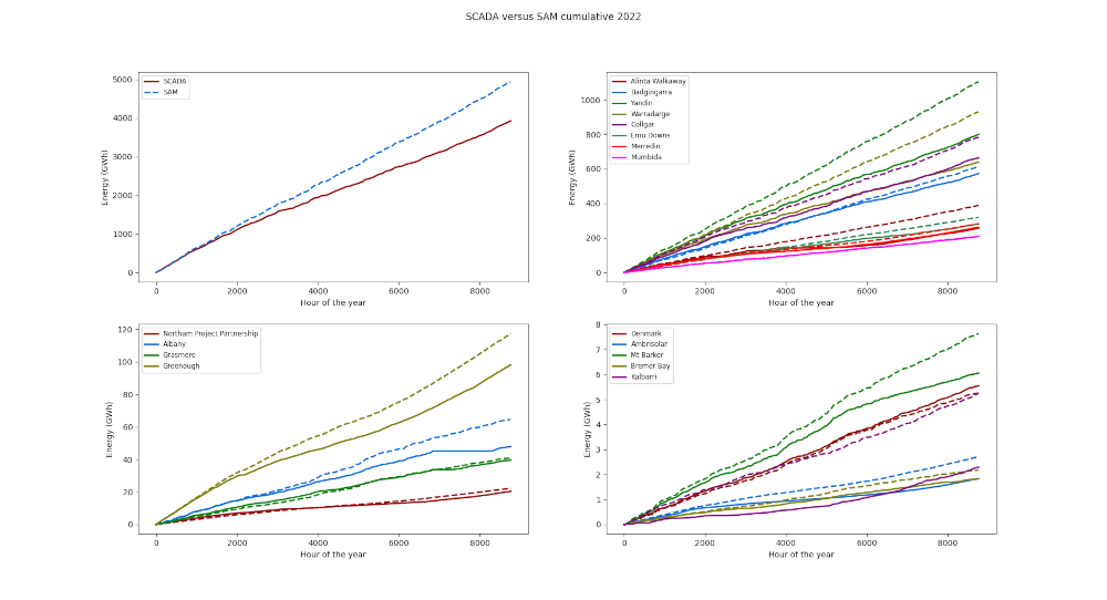
Note: Initially, the swgnt (surface net downward shortwave flux) MERRA variable was used to generate the solar weather variables. This produced outputs that were slightly lower than observed data. To compensate for this a losses percentage of 5 (percent) was used for the SAM pvwattsv5 model. Subsequent work has identified the swgdn (surface incoming shortwave flux) MERRA-2 variable as a more appropriate resource. Using this variable, a losses percentage of 14 - the SAM default - can be used. Validation using either variable (swgnt and 5%, or swgdn and 14%) produces essentially identical results and correlations.

Produce wind and solar weather files

makeweatherfiles

makeweatherfiles is a program that can be used to produce solar and/or wind weather files for input to SAM. The program generates SMW (preferred for SAM) or CSV format solar resource files and SRW format wind resource files. These file formats have been chosen as they're easier to generate than other formats. Using the program you specify the source folder for either the ERA5 or MERRA-2 data files, the time zone for the area of interest, a file format and target folder for the weather files. The program will generate files for each of the ERA5 or MERRA-2 grid squares within the chosen data files or optionally for a number of latitude and longitude positions. You can invoke the program either by choosing makeweatherfiles from the SIREN Tools menu or in Windows by running makeweatherfiles.exe in the siren (or makeweatherfiles) folder. Running it with no parameters will present an interactive window to simplify passing parameters to the tool. The window fields are:

• Year. Year of interest. The naming conventions for MERRA-2 files include the date so this defines the date range. The tool processes dates from the last day of the prior year through to the first day of the next year (ignoring 29 February)
• Wrap to prior year. To enable you to use (more) recent weather data this option will indicate that weather data should wrap to the prior year. As an example, if you have downloaded data up until April for the current year makeweatherfiles will use weather data from the prior year for May onwards to give a full year of data. The data for both years must reside in the same folder (or the next sub-folder if yearly folders are used) and have the same dimensions for latitude and longitude
• Ignore data gaps. This option will cater for individual MERRA-2 files containing different dimensions for latitude and longitude. If this option is selected the program will create weather files where there are gaps for 21 days or less. If there are more gaps the file will not be created.
  • MERRA-2
    • The program does require a MERRA-2 file for each day of the year (It is possible to copy another file, say for the same day of another year, and rename it to “replace” the missing file)
    • In creating a solar weather file the program requires both wind and solar MERRA-2 files, so any gaps in either dataset will result in a gap in the solar weather file
  • ERA5
    • The program requires a ERA5 file for each month of the year
• Time Zone. The (solar) time zone for the area of interest. This is used to create suitable weather files where the first hour in the file is the first hour of the year in the local time zone. A value of auto will cause the program to use the (first) longitude and a value of best will cause the program to use the time zone with the most longitude values in the MERRA-2 data files to calculate the time zone
• Solar Format. The solar option can produce weather files in either of two formats - SMW or CSV format. This option allows you to choose your preferred one. SMW format is suitable for SAM while it may have trouble with the CSV format
• Solar Variable. There are two MERRA-2 solar variables to use to create weather files - swgdn or swgnt. The equivalent ERA5 variables are - ssrd and ssr
• Hub height. To extrapolate wind data above the 50 metre maximum in the MERRA-2 data, or 100 metres in ERA5 data. This can be used to cater for wind turbines with higher hub heights. SAM's windpower model expects wind data within 35 metres of the hub height.
  Note: SIREN can dynamically extrapolate wind data when running Powermodel so if using SIREN there is no need to produce extrapolated wind data
• Extrapolation will use the chosen law, either logarithmic, the default, or Hellmann as described below
• Coordinates. Rather than producing weather files for each grid cell in the chosen area you can restrict it by passing a string of comma-separated latitude and longitude values. The tool will then generate files for just these coordinates.
  • For latitudes and longitudes that don't match cell dimensions in the MERRA-2 files values will be calculated from ratios of values for the surrounding cells
  • If there are data gaps values will be calculated from the nearest cells
• Copy folder down. This is an ease of use field. If this is checked any changes to the Solar Source Folder field will be propagated to the other two Folder fields
• Solar/ERA5 Folder. Use this to specify the location for the MERRA-2 solar (tavg1_2d_rad_Nx) source files or ERA5 data files. To change the location you need to click on the field and navigate to the correct folder (you can't type into the field). This location is used for ERA5 data files and for MERRA-2 it's only used for solar files
• Wind Folder. Use this to specify the location for the MERRA-2 wind (tavg1_2d_slv_Nx) source files. To change the location you need to click on the field and navigate to the correct folder (you can't type into the field). This location is not required for ERA5 data files. For MERRA-2 files it is used for both solar and wind files, so you need to specify it in all cases
• Target Folder. Use this to specify the location for the weather files produced by the tool. To change the location you need to click on the field and navigate to the correct folder (you can't type into the field)

There are six buttons:

• Done will exit the program
• Produce Solar Files will produce solar weather files
• Produce Wind Files will produce wind weather files
• Update Wind Files will update existing wind weather files with extrapolated wind speed
• Help Display this help
• File Info Display details about the weather file dimensions and variables

Creation of weather files may take some time so please be patient. There are two progress bars that will display to indicate how far along the process the program is. The tool will produce an output report which will include the list of weather files produced. The report will include a return code as follows:

• 0. Successful execution
• 1. Successful execution, however, the time zone chosen does not match the time zone(s) suggested by the MERRA-2 data files. If you chose auto or best this indicates more than one time zone is suggested by the MERRA-2 data files
• 2. Error with coordinates field
• 3. Invalid output file format specified. It must be one of csv, smw, srw, or wind
• 4. Data file not found. The program requires filename(s) to be in a specific format so either the filename doesn't match that format or the source folder is incorrect
• 5. Error with data file. If you encounter a MERRA-2 error “Regridder Error. File generation error: Failed to create working directory.” you might attempt to obtain a valid copy of the file in error by entering it's URL entry from the MERRA-2 search results into your browser

You can also run the program on the command line. In this case the parameters are passed to the program as follows:

      makeweatherfiles.exe <parm1=value parm2=value>

Parameters are as described above and can be passed to the program as follows:

• coords= or latlon= A string of comma-separated latitude and longitude values
• extrapolate= or law= The law (model) to extrapolate wind speed data
• fmat= Weather file format
• gaps= A value starting with y (yes) or t (true) indicates to create files with data gaps
• hub_height= A hub height to extrapolate wind speeds
• solar= or erasrc= Location of the ERA5 files or MERRA-2 solar (tavg1_2d_rad_Nx) files
• swg= Solar variable - swgdn or swgnt. Default is swgnt
• target= or tgtdir= Location for the weather files produced
• wind= Location of the MERRA-2 wind (tavg1_2d_slv_Nx) files
• wrap= A value starting with y (yes) or t (true) indicates to wrap back to the prior year
• year= Year of interest
• zone= or timezone= The (solar) time zone for the area of interest

Notes:

1. MERRA-2
   • The program should also handle MERRA (version 1) data files downloaded (probably) prior to February 2016
   • The program assumes each day of data is a separate file and uses the filename to as a “key” to the data. It relies on:
     • The string MERRA being part of the filename
     • Filenames contain tavg1_2d_slv_Nx.YYYYMMDD for wind and tavg1_2d_rad_Nx.YYYYMMDD for solar, where YYYYMMDD indicates the data file for that day
     • All files of the same type (solar or wind) being in the same folder
     • If you download two copies of the same file wget will append a number to the second copy filename, e.g. ...nc4.1. At present these will be ignored
2. ERA5
   • Normally, the program assumes each month of data is a separate file and uses the filename as a “key” to the data. Filenames are of the format era5_data_<yyyymm>.nc
   • It is also possible to use a single file for a year, of the format era5_data_<yyyy>.nc
   • When processing the data the program also looks for data for the last day of the prior year (for timezones > 0) or the first day of the next year (for timezones < 0). It will look for one of the appropriate month file, the appropriate year file, or a file for the single day (era5_data_<yyyymmdd>.nc format)
3. A packaged version of makeweatherfiles for Windows is available as a self-extracting zip file from https://sourceforge.net/projects/sensiren/. The file is sen_makeweather_getera.exe (the package has been created with PyInstaller) and contains makeweatherfiles, getera5, which enables ERA5 files to be downloaded, and getmerra2, which enables MERRA-2 files to be downloaded. This package allows you to create SAM weather files from ERA5 or MERRA-2 files without requiring any other parts of SIREN
4. With increasing hub heights associated with larger turbines the SAM models are impacted by the lack of suitable wind speed data at greater heights. The MERRA-2 climate data has a maximum wind speed height of 50 metres which will cope with hub heights up to around 85 metres. The ERA5 data has a maximum wind speed height of 100 metres which will cope with hub heights up to around 135 metres. To overcome the wind data limitation the Hub height parameter can be used to extrapolate wind speeds to a greater (hub) height. makeweatherfiles will extrapolate wind speed using either of two commonly used laws (models). The law to be used can be specified in the extrapolate property of the [makeweatherfiles] Section of the getfiles.ini Preferences file, and can be either logarithmic, the default, or Hellmann. This additional data will be added to the normal wind file.

   Discussions on the two wind profile laws can be found at ‘Wind profile power law’ (aka Hellmann law; https://en.wikipedia.org/wiki/Wind_profile_power_law) and ‘Log wind profile’ (aka logarithmic law; https://en.wikipedia.org/wiki/Log_wind_profile). The Hellmann law tends to give slightly higher wind speeds. ‘Methodologies Used in the Extrapolation of Wind Speed Data at Different Heights and Its Impact in the Wind Energy Resource Assessment in a Region’ (https://www.researchgate.net/publication/221912731_Methodologies_Used_in_the_Extrapolation_of_Wind_Speed_Data_at_Different_Heights_and_Its_Impact_in_the_Wind_Energy_Resource_Assessment_in_a_Region) provides a fuller discussion on the topic.

Using getera5, getmerra2 and makeweatherfiles

To make use of getera5, getmerra2 and makeweatherfiles the following steps should help:

• getera5 get ERA5 data
  1. Ensure you create a CDS account as described above to gain access to the ERA5 data

  2. Set up a .cdapirc file and for Windows a HOME environment variable. The first time you invoke getera5 it will allow you to set these up

  3. Run getera5 to get the ERA5 data for your area of interest
     1. You specify the bounding coordinates for your area of interest. For example, for the SWIS in Western Australia you could input North -26.0, South -36.0, West 113.125 and East 122.5
     2. Specify the month range. To create a SAM weather file you need at least one year of data plus the last day of the prior year and/or the first day of the next year. As an example Start month: 01/15 (or 2015-01) and End month: 12/15 (or 2015-12) will download data for 2016. ERA5 data is based upon UTC while SAM files are local time. In the case of the SWIS, UTC+8, the first 8 hours of the year will be in the last day of the previous year; for UTC-n, the last n hours of the year will be in the first day of the next year. When you request the data getera5 will check if the file for the required extra day exists and if not it will submit an additional request for the single day of data
     3. Click on the target folder field to specify a location for the ERA5 data
     4. Click Get Data to submit the request. When you click the buttons getera5 will launch separate tasks to download the required files into the target folder. You can Quit out of getera5 as this stage. The tasks will probably take a while to run as they have to request and download individual files for each month or the full year. The output and success will be in a log file in the target folder
     5. If you click Check Data getera5 will interrogate ERA5 files in the appropriate Target Folder to provide the boundaries for the Area of Interest and set the starting date to download the next month in sequence. The interrogation will cater for files in yearly sub-folders

  4. Once the ERA5 files are downloaded run makeweatherfiles to create the SAM weather files

• getmerra2 get MERRA-2 data
  1. Ensure you Register for access as described above to gain access to the MERRA-2 data

  2. Set up a .netrc file and for Windows a HOME environment variable. The first time you invoke getmerra2 it will allow you to set these up

  3. Run getmerra2 to get the MERRA-2 data for your area of interest
     1. You specify the bounding coordinates for your area of interest. For example, for the SWIS in Western Australia you could input North -26.0, South -36.0, West 113.125 and East 122.5. The area has to be at least 1 degree of latitude high by 1.25 degree longitude wide
     2. Specify the date range. To create a SAM weather file you need at least one year of data plus the last day of the prior year and/or the first day of the next year. As an example Start date: 31/12/15 (or 2015-12-31) and End date: 01/01/17 (or 2017-01-01) will download data for 2016. MERRA-2 data is based upon UTC while SAM files are local time. In the case of the SWIS, UTC+8, the first 8 hours of the year will be in the last day of the previous year; for UTC-n, the last n hours of the year will be in the first day of the next year
     3. Click on the target folder field to specify a location for the MERRA-2 data. It's OK to store both wind and solar files in the same folder
     4. Click Get Solar for solar files and Get Wind for wind files. If you're creating solar weather files you'll need both. When you click the buttons getmerra2 will launch separate tasks to download the files into the target folder. You can Quit out of getmerra2 as this stage. The two tasks will probably take a while to run as they have to download individual files for each day in the range. The output and success will be in a log file in the target folder
     5. If you click Check Solar or Check Wind getmerra2 will interrogate MERRA-2 solar files in the appropriate Target Folder to provide the boundaries for the Area of Interest and set the starting date to download the next day in sequence. The interrogation will cater for files in yearly sub-folders

  4. Once the MERRA-2 files are downloaded run makeweatherfiles to create the SAM weather files

• makeweatherfiles - create weather files
  1. Specify the year, 2016 in the case above
  2. Click on the source folder(s) to locate the ERA5 or MERRA-2 files. This will be the same as points 3.1 above
  3. Click on Target folder to specify a location for the weather files. It's convenient to use a different folder to the MERRA-2 files
  4. You can click File Info to test if the data files are OK. This reads the first file of the year (e.g. 20160101) and displays the dimensions of the data file. The output shows the latitude and longitude cells covered
  5. Click Produce Solar Files to create solar weather files. Clicking the button will cause makeweatherfiles to create the solar weather files. It will take a while to run so please be patient. There are two progress bars that will display to indicate how far along the process the program is. It will eventually return with an output listing of the files produced
  6. Click Produce Wind Files to create the wind weather files. Same deal as solar

SAM Weather Files

Wind Files

SRW format wind files are one of the formats acceptable to SAM. This format has been chosen as it's easier to generate than other formats. MERRA-2 variables from tavg1_2d_slv_Nx data files are used to create the SRW variables.

• The wind direction and speed variables are both produced using the northward and eastward MERRA-2 Variables for each height
• The 10m variables are only produced if they exist in the MERRA-2 data files

Solar Files

SMW format solar files are one of the formats acceptable to SAM. This format has been chosen as it's easier to generate than other formats. MERRA-2 variables from both tavg1_2d_rad_Nx and tavg1_2d_slv_Nx data files are used to create the SMW variables.

• The wind direction and speed variables are both produced using the northward and eastward MERRA-2 Variables for each height
• DNI is computed using formulae derived from the NREL Centre for Renewable Energy Resources DISC DNI Model
• DHI is computed using formulae derived from the NREL DNI-GHI to DHI Calculator

Background on ERA5

“ERA5 is the fifth generation ECMWF reanalysis for the global climate and weather for the past 8 decades. Data is available from 1940 onwards. ERA5 replaces the ERA-Interim reanalysis.
Reanalysis combines model data with observations from across the world into a globally complete and consistent dataset using the laws of physics. ... Reanalysis does not have the constraint of issuing timely forecasts, so there is more time to collect observations, and when going further back in time, to allow for the ingestion of improved versions of the original observations, which all benefit the quality of the reanalysis product.”

• I interpret each grid is centred on the latitude / longitude for that set of variables, that is, the value extends outwards in all directions from that point. The actual data is point values at the ERA5 grid point (refer Visualisation of regular lat/lon data) so the grids are equally spaced around a data point

Background on MERRA-2

“The Modern Era Retrospective-analysis for Research and Applications, Version 2 (MERRA-2) is a NASA atmospheric data reanalysis for the satellite era using a major new version of the Goddard Earth Observing System Data Assimilation System Version 5 (GEOS-5). MERRA-2 focuses on historical analyses of the hydrological cycle on a broad range of weather and climate time scales, and places the NASA EOS suite of observations in a climate context.”

• Each time-averaged collection consists of a continuous sequence of data averaged over the indicated interval and time stamped with the central time of the interval. For hourly data, for example, these times are 00:30 GMT, 01:30 GMT, 02:30 GMT, etc..
• I interpret each grid is centred on the latitude / longitude for that set of variables, that is, the value extends outwards in all directions from that point

Using other Weather Files

The use of ERA5 or MERRA-2 data for the weather files is not necessary but provides a way of obtaining (gridded) weather data for any geographic area. Any weather files suitable for SAM can be used by SIREN. Weather Data describes these file formats and Weather Data for non-U.S. Locations gives some details on where non-U.S. weather data may be obtained.

SIREN has two approaches for obtaining weather files:

1. Having the geographic location of the file as part of the filename. This option uses filename formats of <location_latitude_longitude_year> and includes files created from MERRA-2 data by makeweatherfiles. The location for weather files for solar and wind are defined by the solar_files and wind_files properties in the [Files] Section of the Preferences file
2. By using an index file. To use other files you need to create index files that contain the latitude, longitude and filename for each weather file, where the filename is relative to the location for the weather files. Index files for solar and wind are defined by the solar_index and wind_index properties. You can either create these files manually or use indexweather to create an index

indexweather

indexweather is a program that can be used to create an index of solar and/or wind weather files for input to SAM. The program generates an index file that contains latitude, longitude and filename for each weather file. It does this by interrogating some of weather file formats supported by SAM - SAM CSV, SMW and SRW - to obtain the three variables. You can invoke the program either by choosing indexweather from the SIREN Tools menu or in Windows by running indexweather.exe in the siren folder. Running it with no parameters will present an interactive window to simplify passing parameters to the tool. The window fields are:

• Solar files. Location of solar weather files
• Solar index. Name and location for solar index file
• Wind files. Location of wind weather files
• Wind index. Name and location for wind index file

There are four buttons:

• Quit will exit the program
• Produce Solar Index will produce a solar index file
• Produce Wind Index will produce a wind index file
• Help Display this help

You can also run the program on the command line. In this case the parameters are passed to the program as follows:

      indexweather.exe <parm1=value parm2=value>

Parameters are as described above and can be passed to the program as follows:

• solar= Location of the solar weather files
• wind= Location of the wind weather files
• target= name of the index file to produce

Visualising Renewable Resource Attributes

To assist with placement of renewable energy stations SIREN can display a grid of renewable resource attributes derived from the SAM format weather files. This feature utilises summary data stored in a file rather than having to process hourly data from the weather files. The weather data values available are:

• DHI (Diffuse). Average daily DHI insolation (W)
• DNI (Normal). Average daily DNI insolation (W). Important for CST and Solar Thermal generation
• GHI (Direct). Average daily GHI insolation (W). Important for PV generation
• Temperature. Average hourly temperature (^oC)
• Wind Speed. Average hourly wind speed at 10m height (m/s)
• Wind @ 50m. Average hourly wind speed at 50m height (m/s). Important for Wind generation

The Resource Grid window allows you to choose the period and weather variable to display and how it will appear on the SIREN map. By default the period can be either the full year, a month or a season. If there are appropriate files you can also display the variable for an hour within a month or a day. The window also has a Next button which allows you to “step” through the weather periods. You can also use Page Down and Page Up to step forward and back through the weather periods.

The resource files, created by makegrid, summarise weather data for each grid cell to avoid having to process each weather file to obtain the data for the desired time period or hour. There are three possible levels of detail:

• Daily By Month (default). These files summarise the average daily figures for a year, month or season. It provides a gross view to see variances at the monthly level. This is a single spreadsheet with a very approximate disk requirement of about 11Kb per cell
• Hourly By Month. These files summarise the average hourly figures for each month. It provides hourly variances at the monthly level. This is a spreadsheet for each month with a very approximate disk requirement of about 190Kb per cell (15Kb per month)
• Hourly By Day. These files have hourly figures for each day. It provides hourly variances at the daily level. This is a spreadsheet for each day with a very approximate disk requirement of about 5.8Mb per cell (15Kb per day). It allows you to visualise the actual movement of weather events (sun, wind fronts) at the expense of significantly larger disk storage requirements

makegrid

makegrid is a program that can be used to create the resource grid file used by SIREN. You can invoke the program either by choosing makegrid from the SIREN Tools menu or in Windows by running makegrid.exe in the siren folder. Running it with no parameters will present an interactive window to allow you to define what file to create. The window fields are:

• Year. Year of interest
• Update year. If this is checked changes to the year selected will be propagated to the two Folder and Resource File fields
• Level of Detail. Specify the resource files to be created. Values are:- Daily By Month, Hourly By Month, or Hourly By Day
• Non-zero minimum. If this is checked the minimum value for all variables other than temperature will be the lowest non-zero value. For example, if this is checked solar variables will show as empty for hours outside of daylight
• Solar Folder. Source folder for the solar weather files
• Wind Folder. Source folder for the wind weather files
Rain Folder. Source folder for the rain weather files (experimental)
• Resource File. Target file. This can be either a CSV or Excel (XLS or XLSX) file. For an Excel file if you append $MM$ to the year in the filename hourly variable values will be produced
• Properties. This is a read only field that is filled in when the file is created. This property should be copied into the [Files] Section of the Preferences file

There are three buttons:

• Quit will exit the program
• Produce Resource File will produce the file
• Help Display this help

After producing the file you may want to copy contents of the Properties field into the [Files] Section of the Preferences file.

You can also run the program on the command line. In this case the parameters are passed to the program as follows:

      makegrid.exe <parm1=value parm2=value>

Parameters are as described above and can be passed to the program as follows:

• year= Year of interest
rain= Location of the rain weather files (experimental)
• nonzero= Passing a parameter of T(rue) will create non-zero minimums; otherwise the minimum value may be zero
• solar= Location of the solar weather files
• wind= Location of the wind weather files
• target= or tgtfil= Resource grid file to be produced

If the source folder(s) contains other CSV files makegrid may fail. If this happens it is probably safer to copy the weather files to a separate folder.

SAM Models used by SIREN

SIREN uses the NREL SAM SDK API (or SSC) for energy calculations. The current SSC version is 206 (Feb 9 2019). This is a collection of tools developed by NREL for creating renewable energy system models. See SAM Simulation Core SDK for details on the SDK. NREL also provide a user-friendly front end, SAM, to facilitate usage of the SAM models. The SAM front end will allow you to progress any modelling by SIREN to a greater level of detail.

The SAM models are very comprehensive and can be quite complex. For example, there are around 200 input variables possible for the Solar Thermal model SIREN uses. To simplify the interface to SAM, SIREN uses a variable file for each technology to store default values for most variables and only requires a minimal number of variables to be set by the user, such as Capacity. The models used by SIREN and their variable files are as follows:

The variables SIREN requires are as follows. Those from the Preferences file are preceded with the Section they are in.
Note: SAM Variables for tcsmolten_salt vary with SAM (SSC) Version

These files are Excel files. It is possible to update the variables by changing the value in the DEFAULT column. If the value is Input that variable is (already) set by SIREN. If you choose to use the changes to SIREN to support larger turbines (rotor diameter > 85) you can set the default value for wind_turbine_hub_ht in the windpower variables file to Input.

Using the full power of SAM

It is possible to use the full capabilities of SAM by one of two methods:

1. Use SAM:
   1. Run the appropriate model and parameters for the station of interest
   2. Save the hourly power generation figures produce by SAM
   3. Update the Power File field for the station to point this file
   4. Rather than running the Power Model SIREN will access this data file to obtain the hourly figures
2. Create a specific variables file for the technology you're interested in
1. Using the existing file as a starting point create you own version of the file. The structure of the file is generally self-explanatory. Most of the file is created from the SDK with an addition DEFAULT column
2. Update the appropriate property in the [SAM Modules] Section of the Preferences file to point to your file
3. SIREN will then use your file to process that technology
4. If you require different options for different stations with the same technology you can use the Save Hourly Data Output option to save the output for each station. Using Generation - from chosen stations you can create a more specific file

     Wave_Height = 0.023 * 0.3048 * (Wind_Speed * 1.94384)2  (0.3048 converts feet to metres, 1.94384 converts knots to m/s)
     Wave_Period = 0.45 * Wind_Speed * 1.94384
     Wave_Power = Wave_Height2 * Wave_Period * Efficiency of technology

     [Other Wave]
     area=<area per MW>
     capital_cost<Capital cost per peak MW>
     efficiency=<technology efficiency>
     o_m_cost=<Operations and Maintenance cost per peak MW>
     formula=pow(0.0070104 * ( wind * 1.94384)**2,2) * 0.45 * wind * 1.94384 * efficiency * .125

Select area on world map

worldwindow can be used with getmap (see Obtaining a Suitable Map Image), getera5 (see Get ERA5 Files) or getmerra2 (see Get MERRA-2 Files) to choose the Area of Interest for a map or for downloading ERA5 or MERRA-2 data. It presents a world map and allows you to choose the area of interest by clicking within the map and updating the area values in the two calling programs

Using worldwindow

To use worldwindow you simply left click in the map the top left corner of the desired Area of Interest and then left click the bottom right corner. worldwindow will display a rectangle on the world map highlighting the desired area and update the Area of Interest in the calling program. To choose a different area just repeat the process.

worldwindow Menu Structure

View	Overlay items on the world map. Those identified with a tick icon can be toggled on or off   Scale Ruler (Ctrl+R) If True Display a Scale Ruler. If you want to move the ruler you need to toggle it off and then back on again   Coordinates Grid (Ctrl+G) Display a grid for every 10 degrees of latitude and longitude   ERA5 / MERRA-2 Grid (Ctrl+M) Display a grid for every ERA5 or MERRA-2 cell. Due to the number of cells (1,440 latitude x 1,440 longitude, or 720 latitude x 576 longitude) this is not very useful unless you zoom in   Show many Areas This will allow input of coordinates for a number of areas. You enter name (optional), upper latitude, west (left) longitude, lower latitude and east (right) longitude separated by commas for each area of interest. This will then update the map highlighting all areas on the map. This option is useful if you want to show a view of several areas of interest. Note: At present you cannot download maps for each area   Save View (Ctrl+V) Save the current view to an image file
Preferences	Edit or display aspects of the getfiles Preferences file. Changes for some variables will take effect immediately on exit from the edit program while others (such as the map) will require you to restart the simulation   Edit Preferences File(Ctrl+E) Edit the getfiles Preferences file. This option invokes a simple text editor to allow the whole file to be edited   Edit Colours (Ctrl+U) Edit colours for the world map   Edit Section Edit a specific Section of the Preferences file. You will be presented with a list of Sections to choose the desired one. The edit program will then present a table of current Properties and their values
Help	Display some help about the program   Help (F1) Display the help for worldwindow. The default help file, help.html, is a standard HTML file which can be displayed with your browser

getfiles Preferences

The getfiles Preferences file contains preferences specifically for worldwindow, the programs using it and a number of the SIREN tools (getera5, getmap, getmerra2, makeweatherfiles, sirenupd, and updateswis). The file resides in the same folder as worldwindow itself.