Assignment 9: Data Labeling and Feature Selection
Overview
Imagine you want to build a classification model for your company. It's not uncommon that you may encounter the following two problems:
- There is no training data available; data labeling may cost you a lot of money and time.
- The number of features is very large, which may not only lead to long training time but also hurt model generalization.
In this assignment, you will learn how to use Active Learning to address the first problem, and learn how to apply a feature selection approach as well as Principal Component Analysis (PCA) to addressing the second one.
After completing this assignment, you should be able to answer the following questions:
Data Labeling
- Why Active Learning?
- How to implement uncertain sampling, a popular query strategy for Active Learning?
- How to solve an ER problem using Active Learning?
Feature Selection
- Why Feature Selection?
- What are typical Feature Selection approaches?
- How does a filter-based feature selection approach work?
- How does PCA work?
- What're the advantages and disadvantages of PCA?
Part 1. Data Labeling
Active learning is a certain type of ML algorithms that can train a high-quality ML model with small data-labeling cost. Its basic idea is quite easy to understand. Consider a typical supervised ML problem, which requires a (relatively) large training dataset. In the training dataset, there may be only a small number of data points that are beneficial to the trained ML model. In other words, labeling the small number of data points is enough to train a high-quality ML model. The goal of active learning is to help us to identify the data points.
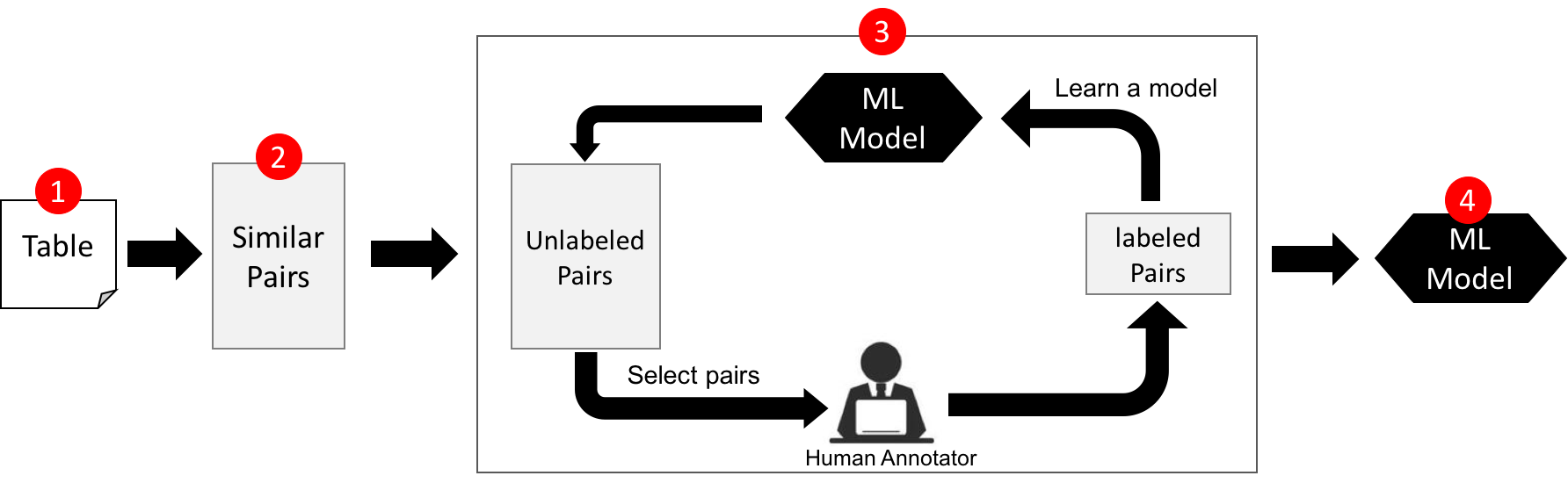
In this assignment, we will revisit Entity Resolution and develop an Active Learning approach for it. Recall that entity Resolution (ER) is defined as finding different records that refer to the same real-world entity, e.g., "iPhone 4-th Generation" vs. "iPhone Four". It is central to data integration and cleaning. The following figure shows the architecture of an entity resolution solution. It consists of four major steps. I will provide you the source code for Steps 1, 2, 4. Your job is to implement Step 3.
Step 1. Read Data
The restaurant data is in a CSV file. Here is the code to read it.
import csv
data = []
with open('restaurant.csv', 'rb') as csvfile:
    reader = csv.reader(csvfile)
    header = reader.next()
    for row in reader:
        data.append(row)
print "Num of Rows:", len(data)
print "Header:", header
print "First Row:", data[0]
print "Second Row:", data[1]
From this dataset, you will find many matching record pairs. For example, the first two rows shown above are matching (i.e., refer to the same real-world entity). You can check out all matching record pairs in the true_matches.json file.
Step 2. Removing Obviously Non-matching Pairs
A naive implementation of entity resolution is to enumerate all $n^2$ pairs and check whether they are matching or not. As you've learnt in Assignment 4, we can avoid $n^2$ comparisons using a similarity-join algorithm.
Here is the code. After running the code, you will get 678 similar pairs ordered by their similarity decreasingly.
from a9_utils import *

simpairs = simjoin(data)

print "Num of Pairs: ", len(data)*(len(data)-1)/2
print "Num of Similar Pairs: ", len(simpairs)
print "The Most Similar Pair: ", simpairs[0]
We can see that simjoin helps us remove the number of pairs from 367653 to 678. But, there are still many non-matching pairs in simpairs (see below).
print simpairs[-1]
Next, we will use active learning to train a classifier, and then use the classifier to classify each pair in simpairs as either "matching" or "nonmatching".
Step 3. Active Learning (Task A)
Given a set of similar pairs, what you need to do next is to iteratively train a classifier to decide which pairs are truly matching. We are going to use logistic regression as our classifier.
Featurization
To train the model, the first thing you need to think about is how to featurize data. That is, transforming each similar pair to a feature vector. Please use the featurize() function for featurization. The function takes a pair as input and returns a vector of 6 features.
from a9_utils import featurize

print "The feature vector of the first pair: ", featurize(simpairs[0])
Initialization
At the beginning, all the pairs are unlabeled. To initialize a model, we first pick up ten pairs and then label each pair using the crowdsourcing() function. You can assume that crowdsourcing() will ask a crowd worker (e.g., on Amazon Mechanical Turk) to label a pair.
crowdsourcing(pair) is a function that simulates the use of crowdsourcing to label a pair
Input: pair – A pair of records
Output: Boolean – True: The pair of records are matching; False: The pair of records are NOT matching;
Please use the following code to do the initialization.
from a9_utils import crowdsourcing

# choose the most/least similar five pairs as initial training data
init_pairs = simpairs[:5] + simpairs[-5:]
matches = []
nonmatches = []
for pair in init_pairs:
    is_match = crowdsourcing(pair)
    if is_match == True:
        matches.append(pair)
    else:
        nonmatches.append(pair)

print "Number of matches: ", len(matches)
print "Number of nonmatches: ", len(nonmatches)
Interactive Model Training
Here is the only code you need to write in Part 1.
from a9_utils import featurize, crowdsourcing


labeled_pairs = matches + nonmatches
unlabeled_pairs = [p for p in simpairs if p not in labeled_pairs]
iter_num = 5

#<-- Write Your Code -->
[Algorithm Description]. Active learning has many query strategies to decide which data point should be labeled. You need to implement uncertain sampling for Task A. The algorithm trains an initial model on labeled_pairs. Then, it iteratively trains a model. At each iteration, it first applies the model to unlabeled_pairs, and makes a prediction on each unlabeled pair along with a probability, where the probability indicates the confidence of the prediction. After that, it selects the most uncertain pair (If there is still a tie, break it randomly), and call the crowdsroucing() function to label the pair. After the pair is labeled, it updates labeled_pairs and unlabeled_pairs, and then retrain the model on labeled_pairs.
[Input].
labeled_pairs: 10 labeled pairs (by default)unlabeled_pairs: 668 unlabeled pairs (by default)iter_num: 5 (by default)
[Output].
model: A logistic regression model built by scikit-learn
[Hints].
- You may need to use logistic regression to train a model.
- You may need to use predict_proba(X) or decision_function(X) to determine which data point should be labeled at each iteration.
Step 4. Model Evaluation
Precision, Recall, F-Score are commonly used to evaluate an entity-resolution result. After training an model, you can use the following code to evalute it.
import json
from a9_utils import evaluate


sp_features = np.array([featurize(sp) for sp in simpairs])
label = model.predict(sp_features)
pair_label = zip(simpairs, label)

identified_matches = []
for pair, label in pair_label:
    if label == 1:
        identified_matches.append(pair)

precision, recall, fscore = evaluate(identified_matches)

print "Precision:", precision
print "Recall:", recall
print "Fscore:", fscore
Part 2. Feature Selection
Feature selection and dimensionality reduction have been extensively studied in the ML community. Due to time constraints, I only designed two simple tasks for you to get familiar with these topics. If you want to know more, please refer to Prof. Michael Jordan's Practical Machine Learning course at UC Berkeley.
Task B. Filter-based Feature Selection
There are three classes of feature-selection methods: filter-based, wrapper-based, and embeded-based. Filter-based is the most simple one. Its basic idea is to assign heuristic score to each feature to filter out the "obviously" useless ones. There are many ways to compute the score, e.g., chi-squared, information gain, correlation, and mutual information. We use chi-squared for Task B.
Imagine you have a collection of newsgroup documents, and you want to build a classification model to predicate the topic of each newsgroup document: "comp.graphics (0)" or "sci.space (1)". You use bag of words to represent each document. That is, each feature is a single word. I have already helped you load the dataset and generated the feature vectors (see the code below).
from sklearn.datasets import fetch_20newsgroups
from sklearn.feature_extraction.text import TfidfVectorizer


data_train = fetch_20newsgroups(subset='train', categories=['comp.graphics','sci.space'],
                                shuffle=True, random_state=42,
                                remove=('headers', 'footers', 'quotes'))

vectorizer = TfidfVectorizer()
X = vectorizer.fit_transform(data_train.data)
y = data_train.target

print "Target Labels:", data_train.target_names
print "(NSamples, NFeatures):", X.shape
From the output of the above code, you find that the number of features (19493) is very large, so you want to use filter-based method to choose the top-10 words as your features.
Please write your code below. The code computes chi-squared stat between each feature and the target label, and return the top-10 words with the highest score.
from sklearn.feature_selection import SelectKBest, chi2

#<-- Write Your Code -->
Task C. Principal Component Analysis (PCA)
PCA is a well-known dimensionality reduction algorithm. Obviously, we can use PCA to transform each feature vector to a 10-D feature vector. See the code below.
import numpy as np
from sklearn.decomposition import PCA

pca = PCA(n_components=10)
pca.fit(X.toarray())
print pca.explained_variance_ratio_
Both filter-based feature selection and PCA can help us reduce the number of features in a feature vector. The question is what's the difference between them. In this task, you don't need to write any code. Just let me know what you think about the advantages and disadvantages of PCA compared to filter-based feature section. Please list (at least) two advantages and two disadvantages.
Submission
Download A9.zip. For Task A and Task B, please directly write your code on the A9.ipynb notebook. For Task C, please write your answers to a file named "PCA.txt". Create a zip package, named A9-final.zip, with the updated A9.ipynb, the newly added "PCA.txt", and three existing files (restaurant.csv, true_matches.json, and a9_utils.py) inside. Please submit A9-final.zip to the CourSys activity Assignment 9.