\title{(some) LaTeX environments \par for Jupyter notebook} \author{@jfbercher} \maketitle
Introduction
This extension for IPython 4.x or Jupyter enables to use some LaTeX commands and environments in the notebook's markdown cells.
\begin{enumerate} \item **LaTeX commands and environments** \begin{itemize} \item support for some LaTeX commands within markdown cells, *e.g.* `\textit`, `\textbf`, `\underline`, `author`, `\title`, LaTeX comments \item support for **theorems-like environments**, support for labels and **cross references** \item support for **lists**: *enumerate, itemize*, \item limited support for a **figure environment**, \item support for an environment *listing*, \item additional *textboxa* environment \end{itemize} \item **Citations and bibliography** \begin{itemize} \item support for `\cite` with creation of a References section \end{itemize} \item it is possible mix markdown and LaTeX markup \item **Document-wide numbering of equations and environments, support for `\label` and `\ref`** \item **Configuration toolbar** \item **LaTeX_envs dropdown menu for a quick insertion of environments** \item Support for **User $\LaTeX$ definitions file** \item Environments title/numbering can be customized by users in ``user_envs.json`` config file \item **Export to plain HTML, Slides and LaTeX with a customized exporter** \item Styles can be customized in the `latex_env.css` stylesheet \item **Autocompletion** for \$, (, {, [, for LaTeX commands and environments \end{enumerate}A simple illustration is as follows: one can type the following in a markdown cell
\begin{listing} The dot-product is defined by equation (\ref{eq:dotp}) in theorem \ref{theo:dotp} just below: \begin{theorem}[Dot Product] \label{theo:dotp} Let $u$ and $v$ be two vectors of $\mathbb{R}^n$. The dot product can be expressed as \begin{equation} \label{eq:dotp} u^Tv = |u||v| \cos \theta, \end{equation} where $\theta$ is the angle between $u$ and $v$ ... \end{theorem} \end{listing}and have it rendered as
The dot-product is defined by equation (\ref{eq:dotp}) in theorem \ref{theo:dotp} just below:
\begin{theorem}[Dot Product] \label{theo:dotp} Let $u$ and $v$ be two vectors of $\mathbb{R}^n$. The dot product can be expressed as \begin{equation} \label{eq:dotp} u^Tv = |u||v| \cos \theta, \end{equation} where $\theta$ is the angle between $u$ and $v$ ... \end{theorem}What's new 
December 2, 2018 - version 1.4.5
- corrected two small issues in LaTeX templates
- added the possibility to "protect" authors in bibTeX reference, issue #41
- corrected a small issue in the optional removing of
toc2toc-cell
February 24, 2018 - version 1.4.2
- @jfbercher Add export to slides with lenvs
jupyter nbconvert --to slides_with_lenvs FILE.ipynb - @jfbercher Corrected inclusion of
latexdefs.texwhen exporting to html - @olehwaa Include notebook figures generated with matplotlib format set to notebook
- @jcb91 add fontawesome css to
latex_envs_toc.tpl(needed for collapsible section icons) - @jfbercher Added system option and per document toggle for autocompletion of
'\$\$','()','{}',''[]' - camaro@octavia Include notebook figures generate when matplotlib format is set to notebook. This generates a png image in in a text/html cell. This image is copied into a image/png cell in the preprocessor, such that it will be recognized by nbconvert as a figure.
- @jfbercher Fix toolbar buttons labels for Jupyter version 5.2+
- @jcb91 use traitlets >= 4.1 tag API, and alias over (deprecated) shortname
- @jfbercher replace
\$\$.\$\$by LaTeX begin-end equation- bib: enable to use \cref, \xref in addition to standard \ref
- bib: add YEAR field if only DATE exists
-add comment environment
- add 5.x compatibility
- @ZrkBreizh Update bibtex2.js
- @olehwaa New method for generating figure captions in latex
- @jfbercher Add autocomplete for LateX commands and environments
- @jfbercher Add a list of environments for which the optional env parameter is not displayed -- case of [H] optional parameter for Figure environment
February 9, 2017 - version 1.3.7
- Enable customizing hotkeys for inserting environments (via
nbextensions_configurator) - LaTeX_envs menu can be customized by editing
envsLatex.jsoninnbextensions/latex_envsdirectory) - Autocompletion for \$,(,{,[
- Updates to ensure compatibility with nbTranslate
- Recognize \ [..\ ] and \ (..\ ) as LaTeX equations delimiters in nb
November 2, 2016 - version 1.3.1
- Support for user environments configuration file (
user_envs.jsoninnbextensions/latex\_envsdirectory). This file is included by the html export template. - Support for book/report style numbering of environments, e.g. "Example 4.2" is example 2 in section 4.
- Support for
\author,\title, andmaketitle. Author and title are saved in notebook metadata, used in html/latex exports. The maketitle command also formats a title in the LiveNotebook. - Added a Toogle menu in the config toolbar to:
- toggle use of user's environments config file
- toggle
report-stylenumbering
September 18, 2016 - version 1.3
- Support for user personal LaTeX definitions file (
latexdefs.texin current directory). This file is included by the html and latex export templates. - Style for nested enumerate environments added in
latex_envs.css - Added a Toogle menu in the config toolbar to:
- toggle the display of the LaTeX_envs dropdown menu,
- toggle the display of labels keys,
- toggle use of user's LaTeX definition file
- Cross references now use the true environment number instead of the reference//label key. References are updated immediately. This works document wide and works for pre and post references
- Support for optional parameters in theorem-like environments
- Support for spacings in textmode, eg
\par,\vspace, \hspace - Support for LaTeX comments % in markdown cells
- Reworked loading and merging of system/document configuration parameters
August 28, 2016 - version 1.2
Added support for nested environments of the same type. Nesting environments of different type was already possible, but there was a limitation for nesting environments of the same kind; eg itemize in itemize in itemize. This was due to to the fact that regular expressions are not suited to recursivity. I have developped a series of functions that enable to extract nested environments and thus cope with such situations.
Corrected various issues, eg #731, #720 where the content of nested environments was incorrectly converted to markdown.
Completely reworked the configuration toolbar. Re-added tips.
- Added a toggle-button for the LaTeX_envs menu
- Added system parameters that can be specified using the nbextensions_configurator. Thus reworked the configuration loading/saving.
- Reworked extension loading. It now detects if the notebook is fully loaded before loading itself.
August 03, 2016 - version 1.13
- Added a template to also keep the toc2 features when exporting to html:
jupyter nbconvert --to html_toclenvs FILE.ipynb Added a dropdown menu that enables to insert all main LaTeX_envs environments using a simple click. Two keybards shortcuts (Ctrl-E and Ctrl-I) for equations and itemize are also provided. More environments and shortcuts can be added in the file
envsLatex.js.Added a link in the general help menu that points to the documentation.
July 27, 2016 - version 1.1
- In this version I have reworked equation numbering. In the previous version, I used a specialized counter and detected equations rendering for updating this counter. Meanwhile, this feature has been introduced in
MathJaxand now we rely on MathJax implementation. rendering is significantly faster. We still have keep the capability of displaying only equation labels (instead of numbers). The numbering is automatically updated and is document-wide. - I have completely reworked the notebook conversion to plain $\LaTeX$ and html. We provide specialized exporters, pre and post processors, templates. We also added entry-points to simplify the conversion process. It is now as simple asto convert
jupyter nbconvert --to html_with_lenvs FILE.ipynb
FILE.ipynbinto html while keeping all the features of thelatex_envsnotebook extension in the converted version.
Main features
Implementation principle
The main idea is to override the standard Markdown renderer in order to add a small parsing of LaTeX expressions and environments. This heavily uses regular expressions. The LaTeX expression are then rendered using an html version. For instance \underline {something} is rendered as <u> something </u>, that is \underline{something}. The environments are replaced by an html tag with a class derived from the name of the environment. For example, a definition denvronment will be replaced by an html rendering corresponding to the class latex_definition. The styles associated with the different classes are specified in latex_env.css. These substitutions are implemented in thsInNb4.js.
Support for simple LaTeX commands
We also added some LaTeX commands (e.g. \textit, \textbf, \underline) -- this is useful in the case of copy-paste from a LaTeX document. The extension also supports some textmode spacings, namely \par, \vspace, \hspace as well as \title, \author, maketitle and LaTeX comments % in markdown cells. Labels and cross-references are supported, including for equations.
Available environments
- theorems-like environments: property, theorem, lemma, corollary, proposition, definition,remark, problem, exercise, example,
- lists: enumerate, itemize,
- limited support for a figure environment,
- an environment listing,
- textboxa, wich is a
textboxenvironment defined as a demonstration (see below).
More environments can be added easily in the user_envs config file user_envs.json or directly in the javascript source file thmsInNb4.js. The rendering is done according to the stylesheet latex_env.css, which can be customized.
Automatic numerotation, labels and references
Several counters for numerotation are implemented: counters for problem, exercise, example, property, theorem, lemma, corollary, proposition, definition, remark, and figure are available.
Mathjax-equations with a label are also numbered document-wide.
An anchor is created for any label which enables to links things within the document: \label and \ref are both supported. A limitation was that numbering was updated (incremented) each time a cell is rendered. Document-wide automatic updating is implemented since version 1.3. A toolbar button is provided to reset the counters and refresh the rendering of the whole document (this is still useful for citations and bibliography refresh).
\label{example:mixing} A simple example is as follows, featuring automatic numerotation, and the use of labels and references. Also note that standard markdown can be present in the environment and is interpreted.
The rendering is done according to the stylesheet latex_env.css, which of course, can be customized to specific uses and tastes.
It is now possible to refer to the definition and to the equation by their labels, as in:
\begin{listing} As an example of Definition \ref{def:FT}, consider the Fourier transform (\ref{eq:FT2}) of a pure cosine wave given by $$ x[n]= \cos(2\pi k_0 n/N), $$ where $k_0$ is an integer. \end{listing}As an example of Definition \ref{def:FT}, consider the Fourier transform (\ref{eq:FT2}) of a pure cosine wave given by $$ x[n]= \cos(2\pi k_0 n/N), $$ where $k_0$ is an integer. Its Fourier transform is given by $$ X[k] = \frac{1}{2} \left( \delta[k-k_0] + \delta[k-k_0] \right), $$ modulo $N$.
Bibliography
Usage
It is possible to cite bibliographic references using the standard LaTeX \cite mechanism. The extension looks for the references in a bibTeX file, by default biblio.bib in the same directory as the notebook. The name of this file can be modified in the configuration toolbar. It is then possible to cite works in the notebook, e.g.
The main paper on IPython is definitively \cite{PER-GRA:2007}. Other interesting references are certainly \cite{mckinney2012python, rossant2013learning}. Interestingly, a presentation of the IPython notebook has also be published recently in Nature \cite{shen2014interactive}.
Implementation
The implemention uses several snippets from the nice icalico-document-tools extension that also considers the rendering of citations in the notebook. We also use a modified version of the bibtex-js parser for reading the references in the bibTeX file. The different functions are implemented in bibInNb4.js. The rendering of citations calls can adopt three styles (Numbered, by key or apa-like) -- this can be selected in the configuration toolbar. It is also possible to customize the rendering of references in the reference list. A citation template is provided in the beginning of file latex_envs.js:
var cit_tpl = {
// feel free to add more types and customize the templates
    'INPROCEEDINGS': '%AUTHOR:InitialsGiven%, ``_%TITLE%_\'\', %BOOKTITLE%, %MONTH% %YEAR%.',
    ... etc
The keys are the main types of documents, eg inproceedings, article, inbook, etc. To each key is associated a string where the %KEYWORDS% are the fields of the bibtex entry. The keywords are replaced by the correponding bibtex entry value. The template string can formatted with additional words and effects (markdown or LaTeX are commands are supported)
Figure environment
Finally, it is sometimes useful to integrate a figure within a markdown cell. The standard markdown markup for that is , but a limitation is that the image can not be resized, can not be referenced and is not numbered. Furthermore it can be useful for re-using existing code. Threfore we have added a limited support for the figure environment. This enables to do something like
which renders as
\begin{figure} \centerline{\includegraphics[width=10cm]{example.png}} \caption{\label{fig:example} This is an example of figure included using LaTeX commands.} \end{figure}Of course, this Figure can now be referenced:
\begin{listing} Figure \ref{fig:example} shows a second filter with input $X_2$, output $Y_2$ and an impulse response denoted as $h_2(n)$ \end{listing}Figure \ref{fig:example} shows a second filter with input $X_2$, output $Y_2$ and an impulse response denoted as $h_2(n)$
figcaption
For Python users, we have added in passing a simple function in the latex_envs.py library.
This function can be imported classically, eg from latex_envs.latex_envs import figcaption (or from jupyter_contrib_nbextensions.nbconvert_support.latex_envs import figcaption if you installed from the jupyter_contrib repo).
Then, this function enables to specify a caption and a label for the next plot. In turn, when exporting to $\LaTeX$, the corresponding plot is converted to a nice figure environement with a label and a caption. The figure can be referenced (after export) using the classical \ref{} command.
To enable large and wide figure in $\LaTeX$ open notebook menu View->Cell Toolbar -> Edit metadata, open the cell metadata and set "widefigure" : true
%matplotlib inline
import matplotlib.pyplot as plt
from latex_envs.latex_envs import figcaption
from numpy import pi, sin, cos,arange
figcaption("This is a nice sine wave", label="fig:mysin")
plt.plot(sin(2*pi*0.01*arange(100)))
plt.show()
figcaption("This is a nice cosine wave", label="fig:mycos")
plt.plot(cos(2*pi*0.01*arange(100)))
plt.show()


Sine wave is shown in fig \ref{fig:mysin} and cosine in fig \ref{fig:mycos}.
Other features
- As shown in the examples, eg \ref{example:mixing} (or just below), it is possible to mix LaTeX and markdown markup in environments
- Support for line-comments: lines beginning with a % will be masked when rendering
Support for linebreaks:
\par_, where _ denotes any space, tab, linefeed, cr, is replaced by a linebreakEnvironments can be nested. egg:
which results in
This is an example of nested environments, with equations inside\par
\begin{proof} Demo % This is a comment \begin{enumerate} \item \begin{equation}\label{eq:} \left\{ p_1, p_2, p_3 \ldots p_n \right\} \end{equation} $$ \left\{ p_1, p_2, p_3 \ldots p_n \right\} $$ \item A **nested enumerate** \item second item \begin{enumerate} \item $\left\{ p_1, p_2, p_3 \ldots p_n \right\}$ \item And *another one* \item second item \begin{enumerate} \item $$ \left\{ p_1, p_2, p_3 \ldots p_n \right\} $$ \item second item \end{enumerate} \end{enumerate} \end{enumerate} \end{proof}User interface
Buttons on main toolbar
On the main toolbar, the extension provides three buttons 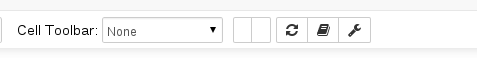 The first one can be used to refresh the numerotation of equations and references in all the document. The second one fires the reading of the bibliography bibtex file and creates (or updates) the reference section. Finally the third one is a toogle button that opens or closes the configuration toolbar.
Configuration toolbar
The configuration toolbar  enables to enter some configuration options for the extension.
First, the LaTeX\_envs title links to this documentation. Then, the bibliography text input can be used to indicate the name of the bibtex file. If this file is not found and the user creates the reference section, then this section will indicate that the file was not found. The References drop-down menu enables to choose the type of reference calls. The Equations input box enables to initiate numbering of equations at the given number (this may be useful for complex documents in several files/parts). The Equations drop-down menu let the user choose to number equation or to display their label instead. The two next buttons enable to toogle display of the LaTeX_envs environments insertion menu or to toggle the displau of LaTeX labels. Finally The Toogles dropdown menu enable to toogle the state of several parameters. All these configuration options are then stored in the notebook's metadata (and restored on reload).
The Toggles dropdown menu
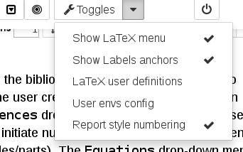
enables to toggle the state of several configuration options:
- display the
LaTeX_envsinsertion menu or not, - show labels anchors,
- use $\LaTeX$ user own LaTeX defintions (loads
latexdefs.texfile from current document directory), - load user's environments configuration (file
user_envs.jsoninnbextensions/latex_envsdirectory), - select "report style" numbering of environments
The LaTeX_envs insertion menu
The LaTeX_envs insertion menu
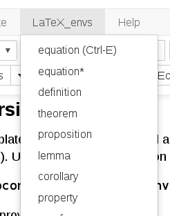 enables a quick insertion of LaTeX environments, some with a keyboard shorcut (this can be customized in
 envsLatex.js). Besides, selected text will be inserted in the environment.
Conversion to LaTeX and HTML
The extension works in the live-notebook. Since it relies on a bunch of javascript, the notebook does not render as is in services such as nbviewer or github viewer. Similarly, nbconvert does not know of the LaTeX constructs which are used here and therefore does not fully convert notebooks using this extension.
Therefore, we provide specialized templates and exporters to achieve these conversions.
Conversion to html
We provide a template latex_envs.tpl and an exporter class LenvsHTMLExporter (in library latex_envs.py). Using that class, conversion simply amounts to
jupyter nbconvert --to latex_envs.LenvsHTMLExporter FILE.ipynbA shortcut is also provided
jupyter nbconvert --to html_with_lenvs FILE.ipynbIt should be noted that the rendering is done exactly in the same way as in the livenotebook. Actually, it is the very same javascript which is run in the html file. The javascript functions are available on the extension github as well as in the jupyter_notebook_extensions CDN, which means that the rendering of the html files requires an internet connection (this is also true for the rendering of equations with MathJax).
Another template latex_envs_toc.tpl is provided which enables to also
keep the toc2 features when exporting to html (it even works if you do not have the toc2 extension!):
jupyter nbconvert --to html_with_toclenvs FILE.ipynb
Finally, it is also possible to embed latex_envs in reveal-js slides. A LenvsHTMLExporter is provided that enables to convert to slides by
jupyter nbconvert --to slidesl_with_lenvs FILE.ipynb
Conversion to LaTeX
We provide two templates thmsInNb_article.tplx and thmsInNb_report.tplx for article and report styles respectively. Anyway one can also use the standard article, report, book templates provided with nbconvert. Simply, we have improved some of the internals styles. More importantly, we provide an exporter class LenvsLatexExporter (also in library latex_envs.py). Using that class, conversion simply amounts to
jupyter nbconvert --to latex_envs.LenvsLatexExporter FILE.ipynbA shortcut is also provided
jupyter nbconvert --to latex_with_lenvs FILE.ipynbIn addition, we provide several further options:
- removeHeaders: Remove headers and footers, (default false)
- figcaptionProcess: Process figcaptions, (default true)
- tocrefRemove Remove tocs and ref sections, + some cleaning, (default true),
These options can be specified on the command line as, eg,
jupyter nbconvert --to latex_with_lenvs --LenvsLatexExporter.removeHeaders=True -- LenvsLatexExporter.tocrefRemove=False FILE.ipynbInstallation
The extension consists in a package that includes a javascript notebook extension. Since Jupyter 4.2, this is the recommended way to distribute nbextensions. The extension can be installed
- from the master version on the github repo (this will be always the most recent version)
- via pip for the version hosted on Pypi
- as part of the great Jupyter-notebook-extensions collection. Follow the instructions there for installing. Once this is done, you can open a tab at
http://localhost:8888/nbextensionsto enable and configure the various extensions.
From the github repo or from Pypi,
- step 1: install the package
pip3 install https://github.com/jfbercher/jupyter_latex_envs/archive/master.zip [--user][--upgrade]- or
pip3 install jupyter_latex_envs [--user][--upgrade] - or clone the repo and install
git clone https://github.com/jfbercher/jupyter_latex_envs.git
python3 setup.py install
With Jupyter >= 4.2,
step 2: install the notebook extension
jupyter nbextension install --py latex_envs [--user]step 3: and enable it
jupyter nbextension enable latex_envs [--user] --py
For Jupyter versions before 4.2, the situation is more tricky since you will have to find the location of the source files (instructions from @jcb91 found here): execute
python -c "import os.path as p; from jupyter_highlight_selected_word import __file__ as f, _jupyter_nbextension_paths as n; print(p.normpath(p.join(p.dirname(f), n()[0]['src'])))"Then, issue
jupyter nbextension install <output source directory>
jupyter nbextension enable latex_envs/latex_envs
where <output source directory> is the output of the python command.
Customization
Configuration parameters
Some configuration parameters can be specified system-wide, using the nbextension_configurator. For that, open a browser at http://localhost:8888/nbextensions/ -- the exact address may change eg if you use jupyterhub or if you use a non standard port. You will then be able to change default values for the boolean values
- LaTeX_envs menu (insert environments) present
- Label equation with numbers (otherwise with their \label{} key)
- Number environments as section.num
- Use customized environments as given in 'user_envs.json' (in the extension directory) and enter a default filename for the bibtex file (in document directory).
All these values can also be changed per documents and these values are stored in the notebook's metadata.
User environments configuration
Environments can be customized in the file user_envs.json, located in the nbextensions/latex_envs directory. It is even possible to add new environments. This file is read at startup (or when using the corresponding toggle option in the Toggles menu) and merged with the standard configuration. An example is provided as example_user_envs.json. For each (new/modified) environment, one has to provide (i) the name of the environment (ii) its title (iii) the name of the associated counter for numbering it; eg
    "myenv": {
        "title": "MyEnv",
        "counterName": "example"
    },
Available counters are problem, exercise, example, property, theorem, lemma, corollary, proposition, definition, remark, and figure.
Styling
The document title and the document author (as specified by \title and \author are formatted using the maketitle command according to the .latex_maintitle and .latex_author div styles.
Each environment is formatted according to the div style .latex_environmentName, e.g. .latex_theorem, .latex_example, etc. The titles of environments are formatted with respect to .latex_title and the optional parameter wrt .latex_title_opt.
Images are displayed using the style specified by .latex_img and thir caption using .caption.
Finally, enumerate environments are formatted according to the .enum style. Similarly, itemize environments are formatted using .item style.
These styles can be customized either in the latex_envs.css file, or better in a custom.css in the document directory.
Usage and further examples
First example (continued)
We continue the first example on fthe Fourier transform definition \ref{def:FT} in order to show that, of course, we can illustrate things using a simple code. Since the Fourier transform is an essential tool in signal processing, We put this in evidence using the textboxa environment -- which is defined here in the css, and that one should define in the LaTeX counterpart:
The Fourier transform of a pure cosine is given by $$ X[k] = \frac{1}{2} \left( \delta[k-k_0] + \delta[k-k_0] \right), $$ modulo $N$. This is illustrated in the following simple script:
%matplotlib inline
import numpy as np
import matplotlib.pyplot as plt
from numpy.fft import fft
k0=4; N=128; n=np.arange(N); k=np.arange(N)
x=np.sin(2*np.pi*k0*n/N)
X=fft(x)
plt.stem(k,np.abs(X))
plt.xlim([0, 20])
plt.title("Fourier transform of a cosine")
_=plt.xlabel("Frequency index (k)")

Second example
This example shows a series of environments, with different facets; links, references, markdown or/and LaTeX formatting within environments. The listing of environments below is typed using the environment listing...
The lines above are rendered as follows (of course everything can be tailored in the stylesheet): %
\begin{definition} \label{def:diffeq} We call \textbf{difference equation} an equation of the form \begin{equation} \label{eq:diffeq} y[n]= \sum_{k=1}^{p} a_k y[n-k] + \sum_{i=0}^q b_i x[n-i] \end{equation} \end{definition}% Properties of the filter are linked to the coefficients of the difference equation. For instance, an immediate property is % % this is a comment
\begin{property} If all the $a_k$ in equation (\ref{eq:diffeq}) of definition \ref{def:diffeq} are zero, then the filter has a **finite impulse response**. \end{property}%
\begin{proof} Let $\delta[n]$ denote the Dirac impulse. Take $x[n]=\delta[n]$ in (\ref{eq:diffeq}). This yields, by definition, the impulse response: \begin{equation} \label{eq:fir} h[n]= \sum_{i=0}^q b_i \delta[n-i], \end{equation} which has finite support. \end{proof}%
\begin{theorem} The poles of a causal stable filter are located within the unit circle in the complex plane. \end{theorem}%
\begin{example} \label{ex:IIR1} Consider $y[n]= a y[n-1] + x[n]$. The pole of the transfer function is $z=a$. The impulse response $h[n]=a^n$ has infinite support. \end{example}In the following exercise, you will check that the filter is stable iff $a$<1. %
\begin{exercise}\label{ex:exofilter} Consider the filter defined in Example \ref{ex:IIR1}. Using the **function** `lfilter` of scipy, compute and plot the impulse response for several values of $a$. \end{exercise}The solution of exercise \ref{ex:exofilter}, which uses a difference equation as in Definition \ref{def:diffeq}:
%matplotlib inline
import numpy as np
import matplotlib.pyplot as plt
from scipy.signal import lfilter
d=np.zeros(100); d[0]=1 #dirac impulse
alist=[0.2, 0.8, 0.9, 0.95, 0.99, 0.999, 1.001, 1.01]
for a in alist:
    h=lfilter([1], [1, -a],d)
    _=plt.plot(h, label="a={}".format(a))
plt.ylim([0,1.5])
plt.xlabel('Time')
_=plt.legend()

Third example:
This example shows that environments like itemize or enumerate are also available. As already indicated, this is useful for copying text from a TeX file. Following the same idea, text formating commands \textit, \textbf, \underline, etc are also available.
which gives...
The following \textit{environments} are available:
\begin{itemize} \item \textbf{Theorems and likes} \begin{enumerate} \item theorem, \item lemma, \item corollary \item ... \end{enumerate} \item \textbf{exercises} \begin{enumerate} \item problem, \item example, \item exercise \end{enumerate} \end{itemize}Disclaimer, sources and thanks
Originally, I used a piece of code from the nice online markdown editor stackedit https://github.com/benweet/stackedit/issues/187, where the authors also considered the problem of incorporating LaTeX markup in their markdown.
I also studied and used examples and code from https://github.com/ipython-contrib/IPython-notebook-extensions.
This is done in the hope it can be useful. However there are many impovements possible, in the code and in the documentation. Contributions will be welcome and deeply appreciated.
If you have issues, please post an issue at
https://github.com/jfbercher/jupyter_latex_envs/issueshere.
Self-Promotion -- Like latex_envs? Please star and follow the repository on GitHub.
%%html
<style>
    .prompt{
        display: none;
    }

</style>
References
(P\'erez and Granger, 2007) P\'erez Fernando and Granger Brian E., ``IPython: a System for Interactive Scientific Computing'', Computing in Science and Engineering, vol. 9, number 3, pp. 21--29, May 2007. online
(McKinney, 2012) Wes McKinney, ``Python for data analysis: Data wrangling with Pandas, NumPy, and IPython'', 2012.
(Rossant, 2013) Cyrille Rossant, ``Learning IPython for interactive computing and data visualization'', 2013.
(Shen, 2014) Shen Helen, ``Interactive notebooks: Sharing the code'', Nature, vol. 515, number 7525, pp. 151--152, 2014.