- Better understand particular details of popular ML algorithms and techniques
- Less code, more insight
- Familiarity with basic statistics and linear algebra concepts assumed
Machine Learning with R - Part II
Ilan Man
Strategy Operations @ Squarespace
Objectives
Agenda
- Logistic Regression
- Principal Component Analysis
- Clustering
Logistic Regression
Objectives
- Motivation
- Concepts and key assumptions
- Approximating parameters
Logistic Regression
Motivation
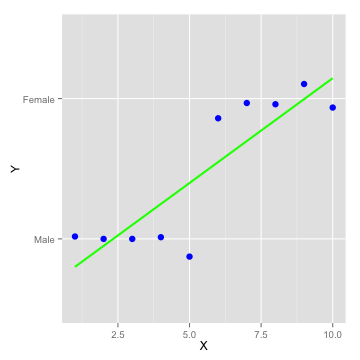
- To model continuous response variables, often turn to linear regression
- \(Price = 500X_{sqr} + 10X_{dist}\)
- Output is (usually) a number
Logistic Regression
Motivation
- To model continuous response variables, often turn to linear regression
- \(Price = 500X_{sqr} + 10X_{dist}\)
- Output is (usually) a number
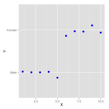
- What about classification problems?
- i.e. male or female, subscribe or not, ...
Logistic Regression
Motivation
Logistic Regression
Motivation
Logistic Regression
Motivation
Logistic Regression
Concepts
- Captures the relationship between a categorical output and some inputs
Logistic Regression
Concepts
- Captures the relationship between a categorical output and some inputs
- \(\hat{y} = \beta_{0} + \beta_{1}x_{1} + ... + \beta_{n}x_{n}\) << Linear Regression
Logistic Regression
Concepts
- Captures the relationship between a categorical output and some inputs
- \(\hat{y} = \beta_{0} + \beta_{1}x_{1} + ... + \beta_{n}x_{n}\) << Linear Regression becomes
- \(\log{\frac{P(Y=1)}{1 - P(Y=1)}} = \beta_{0} + \beta_{1}x_{1} + ... + \beta_{n}x_{n}\)
- "log odds"
- Can be extended to multiple and/or ordered categories
- Probability of rolling a 6 = \(\frac{1}{6}\)
- "Odds for rolling a 6" = \(\frac{P(Y)}{1 - P(Y)} = \frac{\frac{1}{6}}{1-\frac{1}{6}} = \frac{1}{5}\)
Logistic Regression
Concepts
- Family of General Linear Models - GLM
- Random component
- Noise or Errors - Systematic Component
- Linear combination in \(X_{i}\) - Link Function
- Connects Random and Systematic components
- Random component
Logistic Regression
Maximum Likelihood Estimation
- OLS: Minimize the SSE
- MLE: Maximize the (log) likelihood function
- "Given the data, what is the most likely model?"
- MLE satisfies lots of nice properties (unbiased, consistent)
- Used for many types of non-linear regression models
- Complex functions
- Does not require transformation of \(Y\)'s to be Normal
- Does not require constant variance
Logistic Regression
Concepts
- Type of regression to predict the probability of being in a class, say 1 = Female, 0 = Male
- Output is \(P(Y=1\hspace{2 mm} |\hspace{2 mm} X)\)
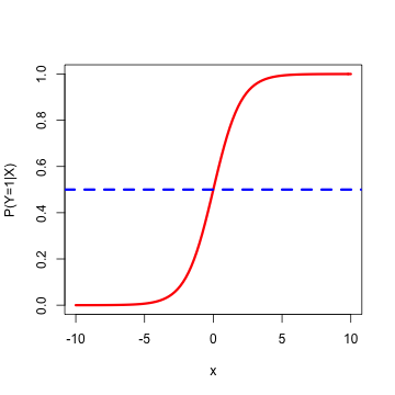
- Typical threshold is 0.5...but it doesn't have to be
Logistic Regression
Concepts
Logistic Regression
Concepts
- Type of regression to predict the probability of being in a class, say 1 = Female, 0 = Male
- Output is \(P(Y=1\hspace{2 mm} |\hspace{2 mm} X)\)
- Typical threshold is 0.5...but it doesn't have to be
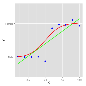
- Sigmoid (logistic) function: \(g(z) = \frac{1}{1+e^{-z}}\)
- Bounded by 0 and 1 (like a probability) for any X
Logistic Regression
Find parameters
- The hypothesis function, \(h_{\theta}(x)\), is \(P(Y=1\hspace{2 mm} |\hspace{2 mm} X)\)
- Linear regression: \(h_{\theta}(x) = \theta^{T}x\)
(Recall that \(\theta^{T}x = \beta_{0} + \beta_{1}x_{1} + ... + \beta_{n}x_{n}\))
Logistic Regression
Find parameters
- The hypothesis function, \(h_{\theta}(x)\), is \(P(Y=1\hspace{2 mm} |\hspace{2 mm} X)\)
- Linear regression: \(h_{\theta}(x) = \theta^{T}x\)
(Recall that \(\theta^{T}x = \beta_{0} + \beta_{1}x_{1} + ... + \beta_{n}x_{n}\)) - Logistic regression: \(h_{\theta}(x) = g(\theta^{T}x)\)
where \(g(z) = \frac{1}{1+e^{-z}}\)
Logistic Regression
Notation
- Re-arranging \(Y = \frac{1}{1+e^{-\theta^{T}x}}\) yields
\(\log{\frac{Y}{1 - Y}} = \theta^{T}x\) - Log odds are linear in \(X\)
Logistic Regression
Notation
- Re-arranging \(Y = \frac{1}{1+e^{-\theta^{T}x}}\) yields
\(\log{\frac{Y}{1 - Y}} = \theta^{T}x\) - Log odds are linear in \(X\)
- This is called the logit of \(Y\)
- Links the odds of \(Y\) (a probability) to a linear regression in \(X\)
- Logit ranges from -ve infite to +ve infinite
- In Linear Regression, when \(x_{1}\) increases by 1 unit, \(Y\) increases by \(\theta_{1}\)
- In Logistic Regression, when \(x_{1}\) increases by 1 unit, \(P(Y=1\hspace{2 mm} |\hspace{2 mm} X)\) increases by \(e^{\theta_{1}}\)
Logistic Regression
Find parameters
- So \(h_{\theta}(x) = \frac{1}{1+e^{-\theta^{T}x}}\)
- To find parameters, minimize cost function
- Use same cost function as for the Linear Regression?
Logistic Regression
Find parameters
- So \(h_{\theta}(x) = \frac{1}{1+e^{-\theta^{T}x}}\)
- To find parameters, minimize cost function
- Use same cost function as for the Linear Regression?
- Logistic residuals are Binomially distributed - not noise
- Regression function is not linear in \(X\); leads to non-convex cost function
Logistic Regression
Find parameters
\[cost(h_{\theta}(x)) = \left\{ \begin{array}{lr} -log(1-h_{\theta}(x)) & : y = 0\\ -log(h_{\theta}(x)) & : y = 1 \end{array} \right. \]


Logistic Regression
Find parameters
- \(Y\) can be Male or Female, 0 or 1 (binary case)
- \(Y \hspace{2 mm} | \hspace{2 mm} X\) ~ Bernoulli
Logistic Regression
Find parameters
- \(Y\) can be Male or Female, 0 or 1 (binary case)
- \(Y \hspace{2 mm} | \hspace{2 mm} X\) ~ Bernoulli
- \(P(Y\hspace{2 mm} |\hspace{2 mm} X) = p\), when \(Y\) = 1
- \(P(Y\hspace{2 mm} |\hspace{2 mm} X) = 1-p\), when \(Y\) = 0
Logistic Regression
Find parameters
- \(Y\) can be Male or Female, 0 or 1 (binary case)
- \(Y \hspace{2 mm} | \hspace{2 mm} X\) ~ Bernoulli
- \(P(Y\hspace{2 mm} |\hspace{2 mm} X) = p\), when \(Y\) = 1
- \(P(Y\hspace{2 mm} |\hspace{2 mm} X) = 1-p\), when \(Y\) = 0
- Joint probability
- \(P(Y = y_{i}|X) = \prod_{i=1}^n p^{y_{i}}(1-p)^{1-y_{i}}\) for many \(y_{i}'s\)
- Taking the log of both sides...
Logistic Regression
Find parameters
- \(P(Y = y_{i}|X) = \prod_{i=1}^n p^{y_{i}}(1-p)^{1-y_{i}}\) for many \(y_{i}'s\)
- \(P(Y = y_{i}|X) = cost(p, y) = - \sum_{i=1}^n y_{i} \log(p) + (1-y_{i}) \log(1-p)\)
Logistic Regression
Find parameters
- \(P(Y = y_{i}|X) = \prod_{i=1}^n p^{y_{i}}(1-p)^{1-y_{i}}\) for many \(y_{i}'s\)
- \(P(Y = y_{i}|X) = cost(p, y) = - \sum_{i=1}^n y_{i} \log(p) + (1-y_{i}) \log(1-p)\)
- \(p = h_{\theta}(x)\)
- \(cost(h_{\theta}(x), y) = -\frac{1}{n}\sum_{i=1}^n y_{i} \log(h_{\theta}(x)) + (1-y_{i}) \log(1-h_{\theta}(x))\)
Logistic Regression
Find parameters
- \(P(Y = y_{i}|X) = \prod_{i=1}^n p^{y_{i}}(1-p)^{1-y_{i}}\) for many \(y_{i}'s\)
- \(P(Y = y_{i}|X) = cost(p, y) = \sum_{i=1}^n -y_{i} \log(p) + (1-y_{i}) \log(1-p)\)
- \(p = h_{\theta}(x)\)
- \(cost(h_{\theta}(x), y) = -\frac{1}{n}\sum_{i=1}^n y_{i} \log(h_{\theta}(x)) + (1-y_{i}) \log(1-h_{\theta}(x))\)
- Minimize the cost
Logistic Regression
Find parameters
- Cannot solve analytically
- Use approximation methods
- (Stochastic) Gradient Descent
- Conjugate Descent
- Newton-Raphson Method
- BFGS
Logistic Regression
Newton-Raphson Method
- Class of hill-climbing techniques
- Efficient
- Easier to calculate than gradient descent
- Except for first and second derivatives
- Fast
Logistic Regression
Newton-Raphson Method

Logistic Regression
Newton-Raphson Method
Logistic Regression
Newton-Raphson Method
Logistic Regression
Newton-Raphson Method
Logistic Regression
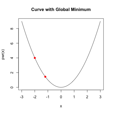
Newton-Raphson Method
- In general, when \(f'(x)\) is \(0\) and \(f''(x) >0\), we've reach a minimum
- Assume \(f'(x_{0})\) is close to zero and \(f''(x_{0})\) is positive
Logistic Regression
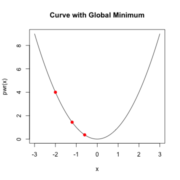
Newton-Raphson Method
- In general, when \(f'(x)\) is \(0\) and \(f''(x) >0\), we've reach a minimum
- Assume \(f'(x_{0})\) is close to zero and \(f''(x_{0})\) is positive
- Re-write \(f(x)\) as its Taylor expansion:
\(f(x) = f(x_{0}) + (x-x_{0})f'(x_{0}) + \frac{1}{2}(x-x_{0})^{2}f''(x_{0})\)
Logistic Regression
Newton-Raphson Method
- In general, when \(f'(x)\) is \(0\) and \(f''(x) >0\), we've reach a minimum
- Assume \(f'(x_{0})\) is close to zero and \(f''(x_{0})\) is positive
- Re-write \(f(x)\) as its Taylor expansion:
\(f(x) = f(x_{0}) + (x-x_{0})f'(x_{0}) + \frac{1}{2}(x-x_{0})^{2}f''(x_{0})\) - Take the derivative w.r.t \(x\) and set = 0
\(0 = f'(x_{0}) + \frac{1}{2}f''(x_{0})2(x_{1} − x_{0})\)
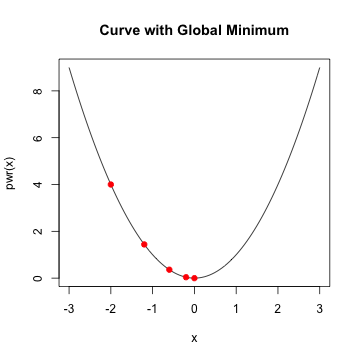
\(x_{1} = x_{0} − \frac{f'(x_{0})}{f''(x_{0})}\)- \(x_{1}\) is a better approximation for the minimum than \(x_{0}\)
- and so on...
Logistic Regression
Newton-Raphson Method
\(f(x) = x^{4} - 3\log(x)\)

Logistic Regression
Newton-Raphson Method
fn <- function(x) x^4 - 3*log(x)
dfn <- function(x) 4*x^3 - 3/x
d2fn <- function(x) 12*x^2 + 3/x^2

newton <- function(num.its, dfn, d2fn){
  theta <- rep(0,num.its)
  theta[1] <- round(runif(1,0,100),0)

  for (i in 2:num.its) {
    h <- - dfn(theta[i-1]) / d2fn(theta[i-1])
    theta[i] <- theta[i-1] + h
  }

  out <- cbind(1:num.its,theta)
  dimnames(out)[[2]] <- c("iteration","estimate")
  return(out)
}
Logistic Regression
Newton-Raphson Method
     iteration estimate
[1,]         1   47.000
[2,]         2   31.333
[3,]         3   20.889
[4,]         4   13.926
[5,]         5    9.284
      iteration estimate
[16,]        16   0.9306
[17,]        17   0.9306
[18,]        18   0.9306
[19,]        19   0.9306
[20,]        20   0.9306
0.9658 ## value of f(x) at minimum
Logistic Regression
Newton-Raphson Method
optimize(fn,c(-100,100)) ## built-in R optimization function
Logistic Regression
Newton-Raphson Method
optimize(fn,c(-100,100)) ## built-in R optimization function
$minimum
[1] 0.9306

$objective
[1] 0.9658
Logistic Regression
Newton-Raphson Method
- Minimization algorithm
- Approximation, non-closed form solution
- Built-in to many programs
- Can be used to find the parameters of a logistic regression equation
Logistic Regression
Summary
- Very popular classification algorithm
- Part of family of GLMs
- Based on Binomial error terms, 1's and 0's
- Assumes linearity between logit function and independent variables
- Uses sigmoid to link the probabilities with regression
Principal Component Analysis
Objectives
- Motivation and examples
- Eigenvalues
- Derivation
- Example
Principal Component Analysis
Motivation
- Unsupervised learning
- Used widely in modern data analysis
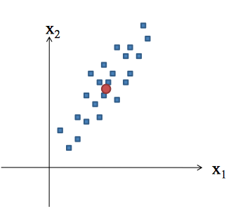
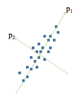
- Compute the most meaningful way to re-express noisy data, revealing the hidden structure
- Commonly used to supplement supervised learning algorithms
Principal Component Analysis
Concepts
Principal Component Analysis
Concepts
Principal Component Analysis
Concepts
Principal Component Analysis
Concepts
Principal Component Analysis
Concepts
Principal Component Analysis
Concepts
Principal Component Analysis
Concepts
Principal Component Analysis
Concepts
Principal Component Analysis
Concepts
Principal Component Analysis
Concepts
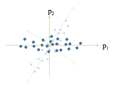
- Assumes linearity
- \(\bf{PX}=\bf{Y}\)
- \(\bf{X}\) is original dataset, \(\bf{P}\) is a transformation of \(\bf{X}\) into \(\bf{Y}\)
- How to choose \(\bf{P}\)?
- Reduce noise (redundancy)
- Maximize signal (variance)
- Provides most information
- Reduce noise (redundancy)
Principal Component Analysis
Concepts
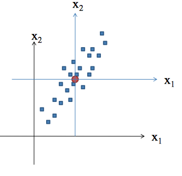
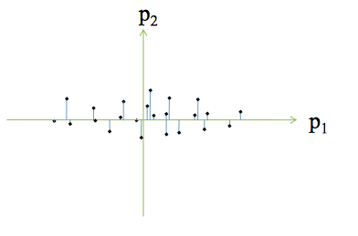
- Covariance matrix is square, symmetric
- \(\bf{C_{x}} = \frac{1}{(n-1)}\bf{XX^{T}}\)
- Diagonals are variances, off-diagonals are covariances
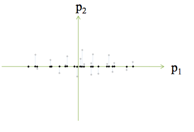
- Goal: maximize diagonals and minimize off-diagonals
- The optimal \(\bf{Y}\) would have a covariance matrix, \(\bf{C_{Y}}\), with positive values on the diagonal and 0's on the off-diagonals
- Diagonalization
Principal Component Analysis
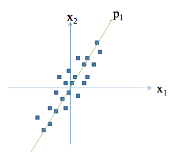
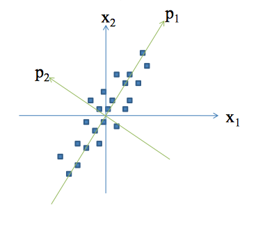
The Objective
- Find some matrix \(\bf{P}\) where \(\bf{PX}=\bf{Y}\) such that \(\bf{Y}\)'s covariance matrix is diagonalized
- The rows of \(\bf{P}\) are the Principal components
- PCA by "eigen decomposition"
Principal Component Analysis
Eigenwhat?
- Eigenvalues help uncover valuable insight into the underlying structure of a vector space
- Eigenvalues/vectors come up extensively in physics, engineering, statistics
- Eigenvalues are scalars derived from a square matrix, "characteristic roots"
- Eigenvectors are non-zero vectors associated with eigenvalues
- Almost every square matrix has at least 1 eigenvalue/vector combo (otherwise its "degenerative")
- Decomposing a square matrix into eigenvalues/vectors is eigen decomposition
Principal Component Analysis
Eigenwhat?
\(\bf{A}x = \lambda x\)
- \(\lambda\) is an eigenvalue of \(\bf{A}\) and \(\bf{x}\) is an eigenvector of \(\bf{A}\)
Principal Component Analysis
Eigenwhat?
\(\bf{A}x = \lambda x\)
\(\bf{A}x - \lambda Ix = 0\)
\((\bf{A} - \lambda I)x = 0\)
For this to be non-trivial \(\det(\bf{A} - \lambda I)\) = 0
- roots are eigenvalues of \(\bf{A}\)
- characteristic polynomial of \(\bf{A}\)
- \({\lambda}\) is called the spectrum
Principal Component Analysis
EigenExample
\[A = \begin{bmatrix} 5 & 2\\ 2 & 5 \end{bmatrix}, I= \begin{bmatrix} 1 & 0\\ 0 & 1 \end{bmatrix}, X = \begin{bmatrix} x_{1}\\ x_{2} \end{bmatrix}\]
Principal Component Analysis
EigenExample
\[A = \begin{bmatrix} 5 & 2\\ 2 & 5 \end{bmatrix}, I= \begin{bmatrix} 1 & 0\\ 0 & 1 \end{bmatrix}, X = \begin{bmatrix} x_{1}\\ x_{2} \end{bmatrix}\] \[\begin{bmatrix} 5 & 2\\ 2 & 5 \end{bmatrix}X = \lambda X\]
Principal Component Analysis
EigenExample
\[A = \begin{bmatrix} 5 & 2\\ 2 & 5 \end{bmatrix}, I= \begin{bmatrix} 1 & 0\\ 0 & 1 \end{bmatrix}, X = \begin{bmatrix} x_{1}\\ x_{2} \end{bmatrix}\] \[\begin{bmatrix} 5 & 2\\ 2 & 5 \end{bmatrix}X = \lambda X\] \[\begin{bmatrix} 5 & 2\\ 2 & 5 \end{bmatrix}X - \lambda X = 0\] \[(\begin{bmatrix} 5 & 2\\ 2 & 5 \end{bmatrix} - \lambda I)X = 0\]
Principal Component Analysis
EigenExample
\[\left | \begin{bmatrix} 5 & 2\\ 2 & 5 \end{bmatrix} - \lambda I \right |= 0\] \[\left|\begin{bmatrix} 5 & 2\\ 2 & 5 \end{bmatrix} - \lambda \begin{bmatrix} 1 & 0\\ 0 & 1 \end{bmatrix} \right| = 0\] \[\left|\begin{bmatrix} 5-\lambda & 2\\ 2 & 5-\lambda \end{bmatrix}\right| = 0\]
Principal Component Analysis
EigenExample
\((5-\lambda)\times(5-\lambda) - 4 = 0\)
\(\lambda^{2} - 10\lambda + 21 = 0\)
\(\lambda = ?\)
Principal Component Analysis
EigenExample
A = matrix(c(5,2,2,5),nrow=2)
roots <- Re(polyroot(c(21,-10,1)))
roots
## [1] 3 7
\(\lambda = 3, 7\)
Principal Component Analysis
Eigencheck
- when \(\lambda = 3\)
\(\bf{Ax} = 3\bf{x}\)
Principal Component Analysis
Eigencheck
- when \(\lambda = 3\)
\(\bf{Ax} = 3\bf{x}\)
\(5x_{1} + 2x_{2} = 3x_{1}\)
\(2x_{1} + 5x_{2} = 3x_{2}\)
Principal Component Analysis
Eigencheck
- when \(\lambda = 3\)
\(\bf{Ax} = 3\bf{x}\)
\(5x_{1} + 2x_{2} = 3x_{1}\)
\(2x_{1} + 5x_{2} = 3x_{2}\)
\(x_{1} = -x_{2}\)
Principal Component Analysis
Eigencheck
- when \(\lambda = 3\)
\(\bf{Ax} = 3\bf{x}\)
\(5x_{1} + 2x_{2} = 3x_{1}\)
\(2x_{1} + 5x_{2} = 3x_{2}\)
\(x_{1} = -x_{2}\)
\[Eigenvector = \begin{bmatrix} 1\\ -1 \end{bmatrix}\]
Principal Component Analysis
Eigencheck
- when \(\lambda = 7\)
\(\bf{Ax} = 7\bf{x}\)
\(5x_{1} + 2x_{2} = 7x_{1}\)
\(2x_{2} + 5x_{2} = 7x_{2}\)
\(x_{1} = x_{2}\)
Principal Component Analysis
Eigencheck
- when \(\lambda = 7\)
\(\bf{Ax} = 7\bf{x}\)
\(5x_{1} + 2x_{2} = 7x_{1}\)
\(2x_{2} + 5x_{2} = 7x_{2}\)
\(x_{1} = x_{2}\)
\[Eigenvector = \begin{bmatrix} 1\\ 1 \end{bmatrix}\]
Principal Component Analysis
Eigencheck
\(\bf{Ax} = \bf{\lambda x}\)
x1 = c(1,-1)
x2 = c(1,1)
A %*% x1 == 3 * x1
A %*% x2 == 7 * x2
Principal Component Analysis
Eigencheck
\(\bf{Ax} = \lambda \bf{x}\)
A %*% x1 == 3 * x1
     [,1]
[1,] TRUE
[2,] TRUE
A %*% x2 == 7 * x2
     [,1]
[1,] TRUE
[2,] TRUE
Principal Component Analysis
Diagonalization
- If \(\bf{A}\) has n linearly independent eigenvectors, then it is diagonalizable
- Written in the form \(\bf{A} = \bf{PD{P}^{-1}}\)
- \(\bf{P}\) is row matrix of eigenvectors
- \(\bf{D}\) is diagonal matrix of eigenvalues of \(\bf{A}\), off-diagonals are 0
- \(\bf{A}\) is "similar"" to \(\bf{D}\)
- Eigenvalues of a symmetric matrix can form a new basis (this is what we want!)
- If the eigenvectors are orthonormal, then \(\bf{{P}^{T} = {P}^{-1}}\)
\(\bf{A} = \bf{PD{P}^{T}}\)
Principal Component Analysis
Diagonalization
\(\bf{A} = \bf{PDP^{T}}\)
m <- matrix(c(x1,x2),ncol=2)  ## x1, x2 are eigenvectors
m <- m/sqrt(norm(m))  ## normalize
as.matrix(m %*% diag(roots) %*% t(m))
##      [,1] [,2]
## [1,]    5    2
## [2,]    2    5
Principal Component Analysis
EigenDecomposition summary
- Eigenvalue and eigenvectors are important
- Linear Algebra theorems allow for matrix manipulation
- Steps to eigendecomposition:
- 1) Set up characteristic equation
- 2) Solve for eigenvalues by finding roots of equation
- 3) Plug eigenvalues back in to find eigenvectors
- But...there's a lot more to eigenvalues!
Principal Component Analysis
Objective
- Find some matrix \(\bf{P}\) where \(\bf{PX}=\bf{Y}\) such that \(\bf{C_{Y}}\) is diagonalized
- Covariance matrix
\(\bf{C_{Y}} = \frac{1}{(n-1)}\bf{YY}^{T}\)
Principal Component Analysis
Proof
\(\bf{PX} = \bf{Y}\)
\(\bf{C_{Y}} = \frac{1}{(n-1)}\bf{YY^{T}}\)
Principal Component Analysis
Proof
\(\bf{PX} = \bf{Y}\)
\(\bf{C_{Y}} = \frac{1}{(n-1)}\bf{YY^{T}}\)
\(=\frac{1}{(n-1)}\bf{PX(PX)^{T}}\)
\(=\frac{1}{(n-1)}\bf{P(XX^{T})P^{T}}\), because \((AB)^{T} = B^{T}A^{T}\)
Principal Component Analysis
Proof
\(\bf{PX} = \bf{Y}\)
\(\bf{C_{Y}} = \frac{1}{(n-1)}\bf{YY^{T}}\)
\(=\frac{1}{(n-1)}\bf{PX(PX)^{T}}\)
\(=\frac{1}{(n-1)}\bf{P(XX^{T})P^{T}}\), because \((AB)^{T} = B^{T}A^{T}\)
\(=\frac{1}{(n-1)}\bf{PAP^{T}}\)
- \(\bf{P}\) is a matrix with rows that are eigenvectors
- \(\bf{A}\) is a diagonalized matrix of eigenvalues and is symmetric...
Principal Component Analysis
Proof
- From earlier, \(\bf{AE} = \bf{ED}\)
- \(\bf{A} = \bf{EDE^{-1}}\)
- Therefore \(\bf{A} = \bf{EDE^{T}}\), because \(\bf{E^{T}}=\bf{E^{-1}}\)
Principal Component Analysis
Motivation
- Choose each row of \(\bf{P}\) to be an eigenvector of \(\bf{A}\)
- Therefore we are forcing this relationship to hold \(\bf{P} = \bf{E^{T}}\)
Principal Component Analysis
Motivation
- Choose each row of \(\bf{P}\) to be an eigenvector of \(\bf{A}\)
- Therefore we are forcing this relationship to hold \(\bf{P} = \bf{E^{T}}\)
Since \(\bf{A} = \bf{EDE^{T}}\)
\(\bf{A} = \bf{P^{T}DP}\)
Principal Component Analysis
Motivation
- Choose each row of \(\bf{P}\) to be an eigenvector of \(\bf{A}\)
- Therefore we are forcing this relationship to hold \(\bf{P} = \bf{E^{T}}\)
Since \(\bf{A} = \bf{EDE^{T}}\)
\(\bf{A} = \bf{P^{T}DP}\)
\(\bf{C_{Y}} = \frac{1}{(n-1)}\bf{PAP^{T}}\)
\(\bf{C_{Y}} = \frac{1}{(n-1)}\bf{P(P^{T}DP)P^{T}}\)
\(\bf{C_{Y}} = \frac{1}{(n-1)}\bf{(PP^{-1})D(PP^{-1})}\)
\(= \frac{1}{n-1}\bf{D}\) - Therefore \(\bf{C_{Y}}\) is diagonalized
Principal Component Analysis
Summary
- The principal components of \(X\) are the eigenvectors of \(XX^{T}\); or the rows of \(P\)
- The \(i^{th}\) diagonal value of \(C_{Y}\) is the variance of \(X\) along
Principal Component Analysis
Assumptions
- Assumes linear relationship between \(\bf{X}\) and \(\bf{Y}\) (non-linear is a kernel PCA)
- Orthogonal components - ensures no correlation among PCs
- Largest variance indicates most signal
- Assumes data is normally distributed, otherwise PCA might not diagonalize matrix
- Can use ICA...
- But most data is normal and PCA is robust to slight deviance from normality
Principal Component Analysis
Example
data <- read.csv('tennis_data_2013.csv')
data$Player1 <- as.character(data$Player1)
data$Player2 <- as.character(data$Player2)

tennis <- data
m <- length(data)

for (i in 10:m){
  tennis[,i] <- ifelse(is.na(data[,i]),0,data[,i])
}
Principal Component Analysis
Example
features <- tennis[,10:m]
dim(features)
## [1] 943 26
str(features)
## 'data.frame':    943 obs. of  26 variables:
##  $ FSP.1: int  61 61 52 53 76 65 68 47 64 77 ...
##  $ FSW.1: int  35 31 53 39 63 51 73 18 26 76 ...
##  $ SSP.1: int  39 39 48 47 24 35 32 53 36 23 ...
##  $ SSW.1: int  18 13 20 24 12 22 24 15 12 11 ...
##  $ ACE.1: num  5 13 8 8 0 9 5 3 3 6 ...
##  $ DBF.1: num  1 1 4 6 4 3 3 4 0 4 ...
##  $ WNR.1: num  17 13 37 8 16 35 41 21 20 6 ...
##  $ UFE.1: num  29 1 50 6 35 41 50 31 39 4 ...
##  $ BPC.1: num  1 7 1 6 3 2 9 6 3 7 ...
##  $ BPW.1: num  3 14 9 9 12 7 17 20 7 24 ...
##  $ NPA.1: num  8 0 16 0 9 6 14 6 5 0 ...
##  $ NPW.1: num  11 0 23 0 13 12 30 9 14 0 ...
##  $ TPW.1: num  70 80 106 104 128 108 173 78 67 162 ...
##  $ FSP.2: int  68 60 77 50 53 63 60 54 67 60 ...
##  $ FSW.2: int  45 23 57 24 59 60 66 26 42 68 ...
##  $ SSP.2: int  32 40 23 50 47 37 40 46 33 40 ...
##  $ SSW.2: int  17 9 15 19 32 22 34 13 14 25 ...
##  $ ACE.2: num  10 1 9 1 17 24 2 0 12 8 ...
##  $ DBF.2: num  0 4 1 8 11 4 6 11 0 12 ...
##  $ WNR.2: num  40 1 41 1 59 47 57 11 32 8 ...
##  $ UFE.2: num  30 4 41 8 79 45 72 46 20 12 ...
##  $ BPC.2: num  4 0 4 1 3 4 10 2 7 6 ...
##  $ BPW.2: num  8 0 13 7 5 7 17 6 10 14 ...
##  $ NPA.2: num  8 0 12 0 16 14 25 8 8 0 ...
##  $ NPW.2: num  9 0 16 0 28 17 36 12 11 0 ...
##  $ TPW.2: num  101 42 126 79 127 122 173 61 94 141 ...
Principal Component Analysis
Example
## Manually Calculated PCs
scaled_features <- as.matrix(scale(features))
Cx <- cov(scaled_features)
eigenvalues <- eigen(Cx)$values
eigenvectors <- eigen(Cx)$vectors
PC <- scaled_features %*% eigenvectors
Cy <- cov(PC)
- Cy should be diagonalized matrix
- diagonals of Cy should be the eigenvalues of Cx
- off diagonals should be 0
Principal Component Analysis
Example
sum_diff <- (sum(diag(Cy) - eigenvalues))^2
round(sum_diff,6)
## [1] 0
off_diag <- upper.tri(Cy)|lower.tri(Cy) ## remove diagonal elements
round(sum(Cy[off_diag]),6)   ## off diagonals are 0 since PC's are orthogonal
## [1] 0
Principal Component Analysis
Example
Principal Component Analysis
Example
pca.df <- prcomp(scaled_features) ## Built in R function
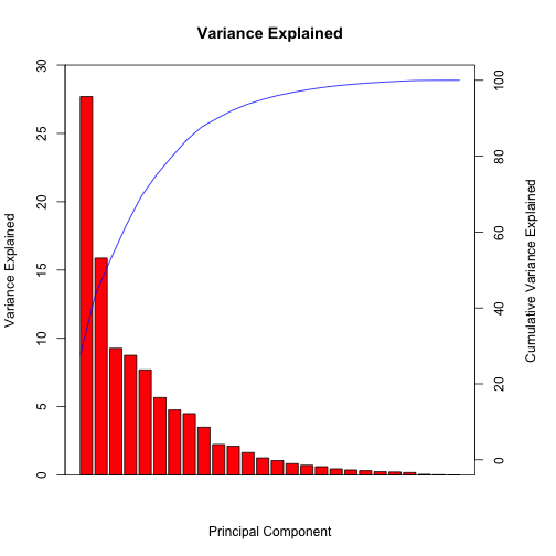
## Eigenvalues of Cx = Variance Explained by PCs
round(eigenvalues,10) == round((pca.df$sdev)^2,10)
 [1] TRUE TRUE TRUE TRUE TRUE TRUE TRUE TRUE TRUE TRUE TRUE TRUE TRUE TRUE
[15] TRUE TRUE TRUE TRUE TRUE TRUE TRUE TRUE TRUE TRUE TRUE TRUE
round(eigenvectors[,1],10) == round(pca.df$rotation[,1],10) ## Eigenvectors of Cx = PCs
FSP.1 FSW.1 SSP.1 SSW.1 ACE.1 DBF.1 WNR.1 UFE.1 BPC.1 BPW.1 NPA.1 NPW.1
 TRUE  TRUE  TRUE  TRUE  TRUE  TRUE  TRUE  TRUE  TRUE  TRUE  TRUE  TRUE
TPW.1 FSP.2 FSW.2 SSP.2 SSW.2 ACE.2 DBF.2 WNR.2 UFE.2 BPC.2 BPW.2 NPA.2
 TRUE  TRUE  TRUE  TRUE  TRUE  TRUE  TRUE  TRUE  TRUE  TRUE  TRUE  TRUE
NPW.2 TPW.2
 TRUE  TRUE
Principal Component Analysis
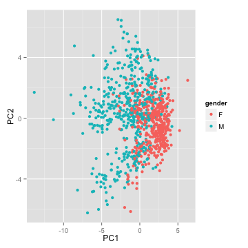
Example
- Can the first two Principal Components separate our data?
Principal Component Analysis
Example
- Classify based on PC1?
PC1 <- pca.df$x[,1]
mean_PC1 <- mean(pca.df$x[,1])
gen <- ifelse(PC1 > mean_PC1,"F","M")
sum(diag(table(gen,as.character(data$Gender))))/rows
[1] 0.7646
Principal Component Analysis
Summary
- Very popular dimensionality reduction technique
- Intuitive
- Cannot reverse engineer dataset easily
- Sparse PCA emphasizes important features
- Non-linear structure is difficult to model with PCA
- Extensions (ICA, kernel PCA) developed to generalize
Clustering
Objectives
- Motivation and examples
- Kmeans
- DBSCAN
Clustering
Motivation
- Separate data into meaningful or useful groups
- Capture natural structure of the data
- Starting point for further analysis
- Cluster for utility
- Summarizing data for less expensive computation
- Data compression
- Very difficult to determine the "correct" number of clusters
Clustering
Types of Clusters
- Data that looks similar
- Prototype based
- Density based
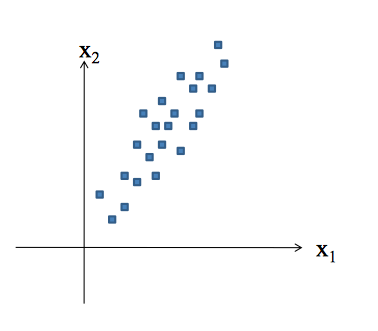
Clustering
Typical clustering problem
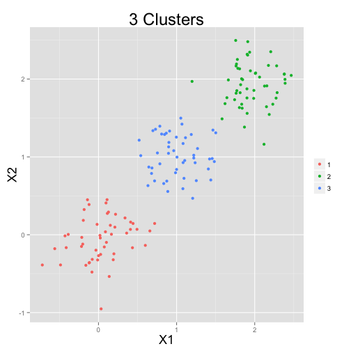
Clustering
Density based cluster

Clustering
Kmeans
- One of the simplest unsupervised learning algorithms
- Group points into clusters; clusters center around a centroid
- Minimize the distance between a point and its centroid
Clustering
Kmeans algorithm
- Select K points as initial centroids
- Do
- Form K clusters by assigning each point to its closest centroid
- Recompute the centroid of each cluster
- Until centroids do not change, or change very minimally, i.e. < 1%
- Computational complexity: \(O(nkI)\)
Clustering
Kmeans algorithm
- Use similarity measures (Euclidean or cosine) depending on the data
- Minimize the squared distance of each point to closest centroid \(SSE(k) = \sum_{i=1}^{m}\sum_{j=1}^{n} (x_{ij} - \bar{x}_{kj})^2\)
Clustering
Kmeans - notes
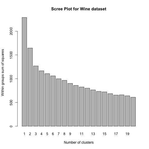
- There is no "correct" number of clusters
- Choose initial K randomly
- Can lead to poor centroids - local minimum
- Run kmeans multiple times
- Reduce the total SSE by increasing K
- Increase the cluster with largest SSE
- Split up a cluster into other clusters
- The centroid that is split will increase total SSE the least
Clustering
Kmeans - notes
- Bisecting Kmeans
- Split points into 2 clusters
- Take cluster with largest SSE - split that into two clusters
- Rerun bisecting Kmeans on resulting clusters
- Stop when you have K clusters
- Less susceptible to initialization problems
Clustering
Kmean fails

Clustering
Kmean fails

Clustering
Kmean fails

Clustering
Kmeans - example
wine <- read.csv('http://archive.ics.uci.edu/ml/machine-learning-databases/wine/wine.data')
names(wine) <- c("class",'Alcohol','Malic','Ash','Alcalinity','Magnesium','Total_phenols',
                 'Flavanoids','NFphenols','Proanthocyanins','Color','Hue','Diluted','Proline')
str(wine[,1:7])
## 'data.frame':    177 obs. of  7 variables:
##  $ class        : int  1 1 1 1 1 1 1 1 1 1 ...
##  $ Alcohol      : num  13.2 13.2 14.4 13.2 14.2 ...
##  $ Malic        : num  1.78 2.36 1.95 2.59 1.76 1.87 2.15 1.64 1.35 2.16 ...
##  $ Ash          : num  2.14 2.67 2.5 2.87 2.45 2.45 2.61 2.17 2.27 2.3 ...
##  $ Alcalinity   : num  11.2 18.6 16.8 21 15.2 14.6 17.6 14 16 18 ...
##  $ Magnesium    : int  100 101 113 118 112 96 121 97 98 105 ...
##  $ Total_phenols: num  2.65 2.8 3.85 2.8 3.27 2.5 2.6 2.8 2.98 2.95 ...
Clustering
Kmeans - example
Clustering
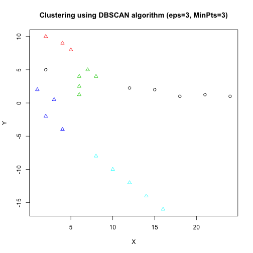
DBSCAN
- A cluster is a dense region of points separated by low-density regions
- Group objects into one cluster if they are connected to one another by densely populated area
- Used when the clusters are irregularly shaped, and when noise and outliers are present
- Computational complexity: \(O(n\log{n})\)
Clustering
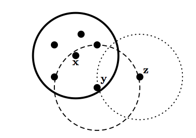
Terminology
- Core points are located inside a cluster
- Border points are on the borders between two clusters
- Neighborhood of p are all points within some radius of p, \(Eps\)
Clustering
Terminology
- Core points are located inside a cluster
- Border points are on the borders between two clusters
- Neighborhood of p are all points within some radius of p, \(Eps\)
Clustering
Terminology
- Core points are located inside a cluster
- Border points are on the borders between two clusters
- Neighborhood of p are all points within some radius of p, \(Eps\)
- High density region has at least \(Minpts\) within \(Eps\) of point p
- Noise points are not within \(Eps\) of border or core points
- If p is density connected to q, they are part of the same cluster, if not, then they are not
- If p is not density connected to any other point, considered noise
Clustering
DBSCAN

Clustering
DBSCAN

Clustering
DBSCAN
Clustering
Summary
- Unsupervised learning
- Not a perfect science - lots of interpretation
- Dependent on values of K, \(Eps\), \(Minpts\)
- Hard to define "correct" clustering
- Many types of algorithms
Summary
ML - Part II
- Logistic regression
- Math behind PCA
- Clustering basics