The philosopher David Lewis described causation as “something that makes a difference, and the difference it makes must be a difference from what would have happened without it.”1 This is the interpretation given to causality by most experimentalists. Even though the definition seems simple, it has many subtle implications. Here are ten ideas implied by this notion of causality that matter for research design.2
For most experimentalists, the statement “\(X\) caused \(Y\)” means that \(Y\) is present and \(Y\) would not have been present if \(X\) were not present. This definition requires a notion of what could have happened, but did not happen.3 Similarly, the “effect” of \(X\) on \(Y\) is thought of as the difference between the value that \(Y\) would have taken given one value of \(X\) and the value that \(Y\) would have taken given another value of \(X\). Because of the focus on differences in outcomes, this approach is sometimes called the “difference making” or “counterfactual” approach to causation.
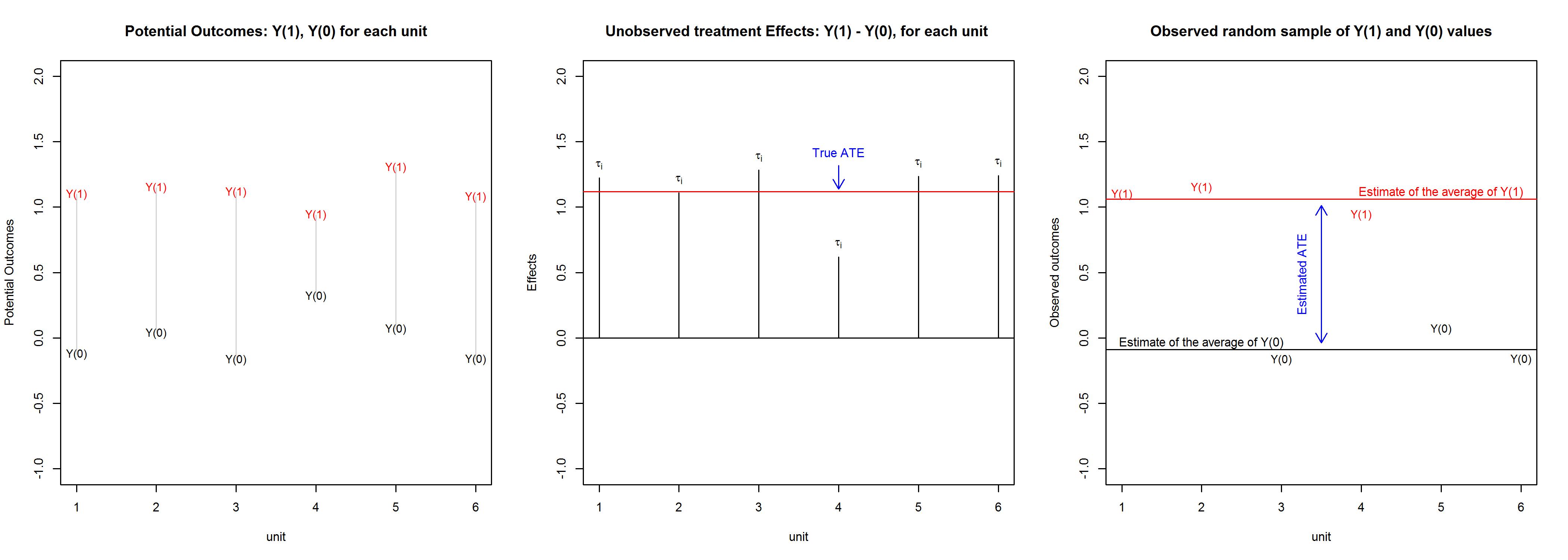
Technical Note: Statisticians employ the “potential outcomes” framework to describe counterfactual relations. In this framework, we let \(Y_i(1)\) denote the outcome for unit \(i\) that would be observed under one condition (e.g., if unit \(i\) received a treatment) and \(Y_i(0)\) the outcome that would be observed in another condition (e.g., if unit \(i\) did not receive the treatment). One causal effect of the treatment for unit \(i\) might be a simple difference of the potential outcomes \(τ_i=Y_i(1)−Y_i(0)\). A treatment has a (positive or negative) causal effect on \(Y\) for unit \(i\) if \(Y_i(1)≠Y_i(0)\).
The “counterfactual” definition of causality requires one to be able to think through what outcomes may result in different conditions. How would things look if one party as opposed to another was elected? Everyday causal statements often fall short of this requirement in one of two ways.
To avoid such problems, some statisticians urge a restriction of causal claims to treatments that can conceivably (not necessarily practically) be manipulated.4 For example, while we might have difficulties with the claim that Peter got the job because he was a man, we have no such difficulties with the claim that Peter got the job because the hiring agency thought he was a man.
Even though we may focus on the effect of a single cause \(X\) on an outcome \(Y\), we generally do not expect that there is ever only a single cause of \(Y\).5 Moreover, if you add up the causal effects of different causes, there is no reason to expect them to add up to 100%. Hence, there is not much point trying to “apportion” outcomes to different causal factors. In other words, causes are not rival. The National Rifle Association argues, for example, that guns don’t kill people, people kill people. That statement does not make much sense in the counterfactual framework. Take away guns and you have no deaths from gunshot wounds. So guns are a cause. Take away people and you also have no deaths from gunshot wounds, so people are also a cause. Put differently, these two factors are simultaneously causes of the same outcomes.
We often talk about causal relations in deterministic terms. Even the Lewis quote at the top of this page seems to suggest a deterministic relation between causes and effects. Sometimes causal relations are thought to entail necessary conditions (for \(Y\) to occur, \(X\) has to happen); sometimes such relations are thought to entail sufficient conditions (if \(X\) occurs, then \(Y\) occurs). But once we are talking about multiple units, there are at least two ways in which we can think of \(X\) causing \(Y\) even if \(X\) is neither a necessary nor a sufficient condition for \(Y\). The first is to reinterpret everything in probabilistic terms: by \(X\) causes \(Y\), we simply mean that the probability of \(Y\) is higher when \(X\) is present. Another is to allow for contingencies — for example, \(X\) may cause \(Y\) if condition \(Z\) is present, but not otherwise.6
If causal effects are statements about the difference between what happened and what could have happened, then causal effects cannot be measured. That’s bad news. Prospectively, you can arrange things so that you can observe either what happens if someone gets a treatment or what happens if they do not get the treatment. Yet, for the same person, you will never be able to observe both of these outcomes and hence also not the difference between them. This inability to observe unit-level causal effects is often called the “fundamental problem of causal inference.”
Even though you cannot observe whether \(X\) causes \(Y\) for any given unit, it can still be possible to figure out whether \(X\) causes \(Y\) on average. The key insight here is that the average causal effect equals the difference between the average outcome across all units if all units were in the control condition and the average outcome across all units if all units were in the treatment condition. Many strategies for causal identification (see 10 Strategies for Figuring Out If X Caused Y) focus on ways to learn about these average potential outcomes.7
10 Things to Know About Hypothesis Testing describes how one can learn about individual causal effects rather than average causal effects given the fundamental problem of causal inference.
One strategy that people use to learn about average causal effects is to create treatment and control groups through randomization (see 10 Strategies for Figuring Out If X Caused Y). When doing so, researchers sometimes worry if they find that the resulting treatment and control groups do not look the same along relevant dimensions.
The good news is that the argument for why differences in average outcomes across randomly assigned treatment and control groups capture average treatment effects (in expectation across repeated randomizations within the same pool of units) does not rely on treatment and control groups being similar in their observed characteristics. It relies only on the idea that, on average, the outcomes in the treated and control groups will capture the average outcomes for all units in the experimental pool if they were, respectively, in treatment or in control. In practice actual treatment and control groups will not be identical.8
A correlation between \(X\) and \(Y\) is a statement about relations between actual outcomes in the world, not about the relation between actual outcomes and counterfactual outcomes. So statements about causes and correlations don’t have much to do with each other. Positive correlations can be consistent with positive causal effects, no causal effects, or even negative causal effects. For example taking cough medication is positively correlated with coughing but hopefully has a negative causal effect on coughing.9
You might expect that if \(A\) causes \(B\) and \(B\) causes \(C\) that therefore \(A\) causes \(C\).10 But there is no reason to believe that average causal relations are transitive in this way. To see why, imagine \(A\) caused \(B\) for men but not women and \(B\) caused \(C\) for women but not men. Then on average \(A\) causes \(B\) and \(B\) causes \(C\) but there may still be no one for whom \(A\) causes \(C\) through \(B\).
Though it might sound like two ways of saying the same thing, there is a difference between understanding what the effect of \(X\) on \(Y\) is (the “effects of a cause”) and whether an outcome \(Y\) was due to cause \(X\) (the “cause of an effect”).11 Consider the following example. Suppose we run an experiment with a sample that contains an equal number of men and women. The experiment randomly assigns men and women to a binary treatment \(X\) and measures a binary outcome \(Y\). Further, suppose that \(X\) has a positive effect of 1 for all men, i.e. men’s control potential outcome is zero (\(Y_i(0) = 0\)) and their treated potential outcome is one (\(Y_i(1) = 1\)). For all women, \(X\) has a negative effect of \(-1\), i.e., women’s control potential outcome is one (\(Y_i(0) = 1\)) and their treated potential outcome is zero (\(Y_i(1) = 0\)). In this example, the average effect of \(X\) on \(Y\) is zero. But for all participants in the treatment group with \(Y=1\), it is the case that \(Y=1\) because \(X=1\). Similarly, for all participants in the treatment group with \(Y=0\), it is the case that \(Y=0\) because \(X=1\). Experimentation can get an exact answer to the question about the “effects of a cause”, but generally it is not possible to get an exact answer to the question about the “cause of an effect”.12
Lewis, David. “Causation.” The journal of philosophy (1973): 556-567.↩︎
Originating author: Macartan Humphreys. Minor revisions: Winston Lin and Donald P. Green, 24 Jun 2016. Revisions MH 6 Jan 2020. Revisions Anna Wilke May 2021. The guide is a live document and subject to updating by EGAP members at any time; contributors listed are not responsible for subsequent edits.↩︎
Holland, Paul W. “Statistics and causal inference.” Journal of the American Statistical Association 81.396 (1986): 945-960.↩︎
Holland, Paul W. “Statistics and causal inference.” Journal of the American Statistical Association 81.396 (1986): 945-960.↩︎
In some accounts this has been called the “Problem of Profligate Causes”.↩︎
Following Mackie, sometimes the idea of “INUS” conditions is invoked to capture the dependency of causes on other causes. Under this account, a cause may be an Insufficient but Necessary part of a condition which is itself Unnecessary but Sufficient. For example dialing a phone number is a cause of contacting someone since having a connection and dialing a number is sufficient (S) for making a phone call, whereas dialing alone without a connection alone would not be enough (I), nor would having a connection (N). There are of course other ways to contact someone without making phone calls (U). Mackie, John L. “The cement of the universe.” London: Oxford Uni (1974).↩︎
Technical Note: The key technical insight is that the difference of averages is the same as the average of differences. That is, using the “expectations operator,” \(𝔼(τ_i)=𝔼(Y_i(1)−Y_i(0))=𝔼(Y_i(1))−𝔼(Y_i(0))\). The terms inside the expectations operator in the second quantity cannot be estimated, but the terms inside the expectations operators in the third quantity can be.7 See illustration here.↩︎
For this reason \(t\)-tests to check whether “randomization worked” do not make much sense, at least if you know that a randomized procedure was followed — just by chance 1 in 20 such tests will show statistically detectable differences between treated and control groups. If there are doubts about whether a randomized procedure was correctly implemented these tests can be used to test the hypothesis that the data was indeed generated by a randomized procedure. This later reason for randomization tests can be especially important in field experiments where chains of communication from the person creating random numbers and the person implementing treatment assignment may be long and complex.↩︎
Technical Note: Let \(D_i\) be an indicator for whether unit \(i\) has received a treatment or not. Then the difference in average outcomes between those that receive the treatment and those that do not can be written as \(\frac{∑_i D_i×Y_i(1)}{∑_iD_i}−\frac{∑_i (1−D_i)×Y_i(0)}{∑_i (1−D_i)}\). In the absence of information about how treatment was assigned, we can say little about whether this difference is a good estimator of the average treatment effect, i.e., of the difference in average treated and control potential outcomes across all units. What matters is whether \(\frac{∑_i D_i×Y_i(1)}{∑_iD_i}\) is a good estimate of \(\frac{∑_i 1×Y_i(1)}{∑_i1}\) and whether \(\frac{∑_i (1−D_i)×Y_i(0)}{∑_i (1−D_i)}\) is a good estimate of \(\frac{∑_i 1×Y_i(0)}{∑_i1}\). This might be the case if those who received treatment are a representative sample of all units, but otherwise there is no reason to expect that it would be.↩︎
Interpret “\(A\) causes \(B\), on average” as “the average effect of \(A\) on \(B\) is positive.”↩︎
Some reinterpret the “causes of effects” question to mean: what are the causes that have effects on outcomes. See Andrew Gelman and Guido Imbens, “Why ask why? Forward causal inference and reverse causal questions”, NBER Working Paper No. 19614 (Nov. 2013).↩︎
See, for example, Tian, J., Pearl, J. 2000. “Probabilities of Causation: Bounds and Identification.” Annals of Mathematics and Artificial Intelligence 28:287–313.↩︎