Choosing α adaptively¶

The module AdaptiveAlpha.py can be used to choose the optimal value of the anisotropy parameter α, with respect to a given optimality criterion and a given family of images.

Currently, the following criteria are implemented:

the asymptotic approximation rate (AAR),
the mean approximation error (MAE),
the thresholding denoising performance (TDP).

In the following, these different criteria are described in greater detail. Finally, we document the auxiliary functions used to implement the criteria.

Documentation of the optimality criteria¶

AdaptiveAlpha.optimize_AAR(image_paths, num_scales, alpha_res, threshold_mode='hard', num_x_values=50, base=1.25, show_plot=True, shearlet_args=None)¶

Given a set of images $f=\{f_1,...,f_N\}$ , this function uses a grid search to determine the optimal value of the parameter alpha of an alpha-shearlet system by comparing the asymptotic approximation rates obtained with different alpha-shearlet systems for the given set of images.

Precisely, the asymptotic approximation rate for a set of images $f=\{f_1,...,f_N\}$ is calculated as follows:

A sequence of threshhold coefficients $c=(c_j)_{j=0,...,J}$ of the form $c_j=c_0\cdot b^{-j}$ is determined, where $c_0>0$ , $b>1$ .
For each of the input images $f_i$ , each alpha and each of the threshold parameters $c_j$ , the approximation error $E_\alpha(f_i;c_j) =\|f_i-S_\alpha^{-1}\Lambda_{c_j}S_\alpha f_i\|_{L^2}$ is calculated. Here, $\Lambda_c$ is a thresholding operator with cut-off (or threshold) $c$ , $S_\alpha$ is the alpha-shearlet transform and $S_\alpha^{-1}$ the (pseudo)-inverse of the alpha-shearlet transform. All images are normalized to satisfy $\|f_i\|_{L^2}=1$ .
The mean of the approximation errors with respect to the image set is taken: $E_\alpha(f;c_j)=\frac{1}{N}\sum_{i=1}^N \|f_i-S_\alpha^{-1}\Lambda_{c_j}S_\alpha f_i\|_{L^2}$ .
For each value of alpha, the logarithm of $E_\alpha(f;c_j)$ , as a function of $j$ , is considered as a time series which is partitioned into almost linear parts using piecewise linear times series segmentation; see common_linear_segmentation() for more details and the techincal report for motivation.
The value of alpha yielding the smallest slope (i.e., the fastest error decay) in the last of these almost linear parts is considered as the optimum.

Many parameters (number of different alpha values, number of threshold parameters, etc.) of the procedure described above can be customized using the parameters of optimize_AAR(). These parameters are described in the following list.

Required parameters

Parameters:

image_paths (list) –
This parameter determines the set of images to be considered. Precisely, image_paths should be a list of strings, where each string is the path of an image, i.e., of a .png or a .npy file.

All of these images/numpy arrays have to be two-dimensional and all of the same dimension. Furthermore, image_paths should contain at least one path.
num_scales (int) – Number of scales which the different alpha-shearlet systems should use.
alpha_res (float) –
This parameter determines the resolution (or density) which is used by the grid search to determine the optimal value of alpha. The different alpha values are taken uniformly over the interval [0,1], with sampling density alpha_res.

Note

If one wants to determine the number of different alpha values, this can be done by passing alpha_res = 1 / (num_alphas - 1), where num_alphas is the desired number of different alpha values.

Keyword parameters

Parameters:

threshold_mode (string) –
Either 'hard' or 'soft'. This parameter determines whether the hard thresholding operator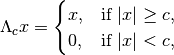

$\Lambda_cx = \begin{cases} x, & \text{if }|x|\geq c, \\ 0, & \text{if }|x|<c, \end{cases}$

or the soft thresholding operator

$\Lambda_cx =\begin{cases} x\cdot \frac{|x|-c}{|x|}, & \text{if }|x|\geq c, \\ 0, & \text{if }|x|<c \end{cases}$

is used for thresholding the alpha-shearlet coefficients.
num_x_values (int) – Number of different threshold parameters that are used. Precisely, the considered thresholds are $(c_j)_{j=0,...,J}$ , with $c_j = c_0 \cdot b^{-j}$ , where $J = \mathrm{num\_x\_values} - 1$ and where the base b is determined by the parameter base. Finally, $c_0$ is choosen as the maximum value of $\|S_\alpha f_i\|_\infty$ over all images and all values of alpha.
base (float) – Value of the basis $b>1$ for the calculation of the threshold parameters $c_j=c_0\cdot b^{-j}$ . See num_x_values for a more thorough explanation.
show_plot (bool) – If this paramter is set to True, executing optimize_AAR() will also display a log-log plot of $E_\alpha (f;c)$ , together with the associated partition into almost linear parts.
shearlet_args (dict) –
This argument can be used to determine the properties of the employed alpha-shearlet systems. A typical example of this argument is:
```
{'subsampled' : False, 'real' : True, 'verbose' : False}
```
where the chosen values of True or False can of course differ.

Note

The parameter shearlet_args is just passed as a set of keyword arguments to the constructor of the class AlphaShearletTransform. See the documentation of that class for more details, in particular for the respective default values.

Return value

Returns:	The function returns that value of alpha (as a `float`) which yields the smallest asymptotic approximation rate, i.e., the fastest asymptotic error-decay, for the given set of images.

AdaptiveAlpha.optimize_MAE(image_paths, num_scales, alpha_res, threshold_mode='hard', num_x_values=50, max_value=None, show_plot=True, shearlet_args=None)¶

Given a set of images $f=\{f_1,...,f_N\}$ , this function uses a grid search to determine the optimal value of the parameter alpha of an alpha-shearlet system by comparing the mean approximation error obtained with different alpha-shearlet systems for the given set of images.

Precisely, the mean approximation error for a set of images $f=\{f_1,...,f_N\}$ is calculated as follows:

A sequence of threshold coefficients $c=(c_j)_{j=1,...,J}$ is determined. In fact, the $c_j$ are chosen to be uniformly distributed in an interval $[0, m]$ , where the maximal value m is determined by the parameter max_value.
For each of the input images $f_i$ , each alpha and each of the threshold parameters $c_j$ , the approximation error $E_\alpha(f_i;c_j)= \|f_i-S_\alpha^{-1}\Lambda_{c_j}S_\alpha f_i\|_{L^2}$ is calculated. Here, $\Lambda_c$ is the (hard) thresholding operator with cut-off (or threshold) $c$ , $S_\alpha$ is the alpha-shearlet transform and $S_\alpha^{-1}$ the (pseudo)-inverse of the alpha-shearlet transform. All images are normalized so that $\|f_i\|_{L^2}=1$ .
The mean of the approximation errors with respect to the image set and with respect to the threshold parameters is taken: $\text{MAE}(f;\alpha)=\frac{1}{N}\sum_{i=1}^N \frac{1}{J} \sum_{j=1}^J\|f_i-S_\alpha^{-1}\Lambda_{c_j}S_\alpha f_i\|_{L^2}$ .
The value of alpha which yields the smallest value for $\text{MAE}(f;\alpha)$ is considered as the optimum.

Many parameters (number of different alpha values, number of threshold parameters, etc.) of the procedure described above can be customized using the parameters of optimize_MAE(). These are described in the following list.

Required parameters

Parameters:

image_paths (list) –
This parameter determines the set of images to be considered. Precisely, image_paths should be a list of strings, where each string is the path of an image, i.e., of a .png or a .npy file.

All of these images/numpy arrays have to be two-dimensional and all of the same dimension. Furthermore, image_paths should contain at least one path.
num_scales (int) – Number of scales which the different alpha-shearlet systems should use.
alpha_res (float) –
This parameter determines the resolution (or density) which is used by the grid search to determine the optimal value of alpha. The different alpha values are taken uniformly over the interval [0,1], with sampling density alpha_res.

Note

If one wants to determine the number of different alpha values, this can be done by passing alpha_res = 1 / (num_alphas - 1), where num_alphas is the desired number of different alpha values.

Keyword parameters

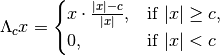
Parameters:

threshold_mode (string) –
Either 'hard' or 'soft'. This parameter determines whether the hard thresholding operator

$\Lambda_cx =\begin{cases} x & \text{if }|x|\geq c\\ 0 & \text{if }|x|<c \end{cases}$

or the soft thresholding operator

$\Lambda_cx =\begin{cases} x\cdot \frac{|x|-c}{|x|} & \text{if }|x|\geq c\\ 0 & \text{if }|x|<c \end{cases}$

is applied to each of the alpha-shearlet coefficients.
num_x_values (int) – Number of different threshold parameters that are used. These are taken equally distributed from $\{0,...,\mathrm{max\_value}\}$ .
max_value (float) –
Maximum value of the threshold parameter.

If the default value (None) is passed, max_value is taken as the largest absolute value of all alpha-shearlet coefficients (maximizing over all images and all considered values of alpha) which do not belong to the low-pass part. The reason for this choice is that if c is chosen greater than this threshold, then $E_\alpha (f_i; c)$ is independent of $\alpha$ .
show_plot (bool) – If this parameter is set to True, executing optimize_MAE() will display a plot of the error curves $E_\alpha (f; c)$ (jointly for all considered alpha values) as a function of c.
shearlet_args (dict) –
This argument can be used to determine the properties of the employed alpha-shearlet systems. A typical example of this argument is:
```
{'subsampled' : False, 'real' : True, 'verbose' : False}
```
where the chosen values of True or False can of course differ.

Note

The parameter shearlet_args is just passed as a set of keyword arguments to the constructor of the class AlphaShearletTransform. See the documentation of that class for more details, in particular for the respective default values.

Return value

Returns:	The function return the value of alpha (as a `float`) which yields the smallest value of $\text{MAE}(f;\alpha)$ for the given set of images.

AdaptiveAlpha.optimize_denoising(image_paths, num_scales, alpha_res, num_noise_lvls, noise_min=0.02, noise_max=0.4, sample_size=None, thresh_multiplier=None, show_plot=True, shearlet_args=None)¶

Given a set of images, this function uses a grid search to determine the optimal value of the parameter alpha of an alpha-shearlet system by comparing the performance of different alpha-shearlet systems for certain denoising experiments using the given set of images.

Precisely, the denoising performance is measured as follows: For each of the input images $f_i$ , the following operations are performed:

Gaussian noise $\mathcal{N} = \mathcal{N}_\sigma$ with standard deviation $\sigma$ is added to $f_i$ to obtain a distorted image $\tilde{f_i} = f_i + \mathcal{N}$ .

Note

Each $f_i$ is actually a normalized version of an input image, i.e., $\|f_i\|_{L^2} = 1$ . This normalization is used to ensure that the standard deviation $\sigma$ is comparable to the image itself.
The alpha-shearlet transform $S_\alpha \tilde{f_i}$ of $\tilde{f_i}$ is computed.
The alpha-shearlet coefficients are thresholded, yielding $\Lambda_c S_\alpha \tilde{f_i}$ , where $\Lambda_c$ is the hard thresholding operator with cut-off (or threshold) c.

The precise value of the threshold c is actually noise- and scale-dependent. See below for a more detailed description.
The thresholded coefficients are used to reconstruct a denoised version $g_i$ of $\tilde{f_i}$ . Precisely, $g_i = S_\alpha^{-1} \Lambda_c S_\alpha \tilde{f_i}$ , where $S_\alpha^{-1}$ is the (pseudo)-inverse of $S_\alpha$ .
The error $\mathrm{TDP}_\alpha (f_i;\sigma) = \|f_i - g_i\|_{L^2}$ is computed to measure the suitability of the alpha-shearlet system for denoising the given image $f_i$ .

This procedure is repeated for all images in the given set and for a number of different noise levels $\lambda$ , where the noise level is proprtional to the standard deviation $\sigma$ of the gaussian noise $\mathcal{N}_\sigma$ . In total, the suitability of the alpha-shearlet system for denoising the given set of images is measured by taking the mean over all given images and all considered noise levels, i.e., by

$\mathrm{TDP}_\alpha ((f_1, \dots, f_N)) & := \frac{1}{N} \sum_{i=1}^N \frac{1}{|\Sigma|} \sum_{\sigma \in \Sigma} \mathrm{TDP}_\alpha (f_i; \sigma),$

where $\Sigma$ denotes the set of all considered standard deviations.

Many parameters (number of different alpha values, number of different noise levels, etc.) of the procedure described above can be customized using the parameters of optimize_denoising(). These are described in the following list.

Required Parameters

Parameters:

image_paths (list) –
This parameter determines the set of images to be considered. Precisely, image_paths should be a list of strings, where each string is the path of an image, i.e., of a .png or a .npy file.

All of these images/numpy arrays have to be two-dimensional and all of the same dimension. Furthermore, image_paths should contain at least one path.
num_scales (int) – Number of scales which the different alpha-shearlet systems should use.
alpha_res (float) –
This parameter determines the resolution (or density) which is used by the grid search to determine the optimal value of alpha. The different alpha values are taken uniformly over the interval [0,1], with sampling density alpha_res.

Note

If one wants to determine the number of different alpha values, this can be done by passing alpha_res = 1 / (num_alphas - 1), where num_alphas is the desired number of different alpha values.
num_noise_lvls (int) – Number of different noise levels that are used. These are taken equally distributed from the interval [noise_min, ..., noise_max].

Keyword parameters

Parameters:

noise_min (float) –
Lower bound for the range from which the different noise levels are taken. Default value is $0.02$ .

Note

The standard deviation $\sigma$ of the noise and the noise level $\lambda$ are related by

$\sigma=\lambda/\sqrt{N_1\cdot N_2},$

where $N_1 \times N_2$ is the common dimension of all considered images. This ensures

$\mathbb{E} \|\mathcal{N}_\sigma\|_{L^2}^2 = N_1 \cdot N_2 \cdot \sigma^2 = \lambda^2,$

so that $\| \mathcal{N}_\sigma\|_{L^2}$ is typically about $\lambda$ . Since we are considering normalized images, $\lambda$ is thus a good measure for the noise to signal ratio.
noise_max (float) – Upper limit for the range from which the different noise levels are taken. Default value is 0.4. See noise_min for more details.
sample_size (int) –
This parameter can be used to test whether generalization occurs, i.e., if the optimal value of alpha learned on a small subset (the training set) of the data yields the same value as for the whole data set.

Precisely, if sample_size is passed a value different from the default (None), then optimize_denoising also determines the optimal value of alpha for a randomly chosen subset of the given images. This randomly chosen subset has sample_size elements, i.e., sample_size determines the size of the training set.
thresh_multiplier (list) –
This parameter determines how the threshold c for the hard thresholding operation is determined as a function of the noise level and of the scale.

Precisely, the coefficients on scale i are thresholded with cutoff value sigma * thresh_multiplier[i+1]. Here, the low-pass has i = -1, while the other scales “begin counting” at i = 0. Furthermore, sigma is the standard deviation of each entry of the noise.

If the default value (None) is used, then thresh_multiplier is chosen as [3] * num_scales + [4], so that all scales but the highest use a cutoff of 3 * sigma, while the highest scale uses 4 * sigma.

Note

One can show (since we use the normalized alpha-shearlet coefficients, i.e., with $\|\psi_i\|_{L^2} = 1$ ) that each coefficient $(S_\alpha \mathcal{N}_\sigma)_i$ is normally distributed with standard deviation $\sigma$ . Hence, choosing the threshold as a multiple of sigma is natural.
show_plot (bool) –
If this parameter is set to True, executing optimize_denoising() will also display a plot of the average denoising error

$\frac{1}{N} \sum_{i=1}^N \mathrm{TDP}_\alpha (f_i ; \sigma)$

as a function of the noise level $\lambda = \sqrt{N_1 \cdot N_2} \cdot \sigma$ in one common plot for all values of alpha.
shearlet_args (dict) –
This argument can be used to determine the properties of the employed alpha-shearlet systems. A typical example of this argument is:
```
{'subsampled' : False, 'real' : True, 'verbose' : False}
```
where the chosen values of True or False can of course differ.

Note

The parameter shearlet_args is just passed as a set of keyword arguments to the constructor of the class AlphaShearletTransform. See the documentation of that class for more details, in particular for the respective default values.

Return value

Returns:

If sample_size is None, this function returns a single float, namely the value of alpha yielding the best denoising performance on the given images.

If sample_size is not None, this function returns a tuple t of two floats, where t[0] is the value of alpha yielding the best denoising performance on all of the given images, while t[1] is the value of alpha yielding the best denoising performance on the randomly selected training set of size sample_size.

Documentation of auxiliary functions¶

AdaptiveAlpha.common_linear_segmentation(list_of_ys, max_error, direction)¶

This function performs a sliding window piecewise linear time series segmentation, based on a certain Stackoverflow post, simultaneously over a given set of time series.

The parameter list_of_ys contains the set of time series, i.e., it is of the form $\mathrm{list\_of\_ys} = [\mathrm{ys}^{(0)}, \dots, \mathrm{ys}^{(N)}]$ , where each element $\mathrm{ys}^{(i)}$ is itself a list with real values $\mathrm{ys}^{(i)} = [y_0^{(i)}, \dots, y_{n-1}^{(i)}]$ , representing a time series. Note that the length n of the time series should be independent of i. The function then computes a sequence $(x_1, ..., x_\ell)$ of break points such that between each pair of consecutive break points, each of the sequences $\mathrm{ys}^{(i)}$ is “almost linear”.

Required parameters

Parameters:

list_of_ys (list) – List of time series (of common length) which will be simultaneously split into “almost linear” parts using a common segmentation. For more details on the form of list_of_ys, see the description from above.
max_error (float) –
A positive real number. The interval $[0, \dots, n]$ , where n is the common length of all time series, is split into a number of intervals (segments) such that on each segment and for each of the time series ys, the best (affine)-linear approximation (in the sense of linear regression) to the time series ys itself has a uniform error of at most max_error * (max(ys) - min(ys)).

Hence, for a given value of max_error, the allowed tolerance is still weighted with the actual spread of the values in each of the time series. This ensures that a segmentation of a scaled version of the given time series will result in the same segmentation as for the original time series.
direction (string) –
Either 'forward' or 'reversed'.

For ordinary sliding window piecewise linear segmentation, one starts at the beginning of the time series (i.e., at 0) and enlarges the current segment until the criterion described above (see max_error) fails; then one starts the next segment. If direction is 'forward', this is exactly what this function does. If direction is 'reversed', then we start at the end of the time series instead of at the beginning.

Return values

Returns:

A tuple (breaks, slopes), where

breaks is a list of nonnegative integers which is of the form $[x_0=0, x_1, ..., x_{k},x_{\ell+1}=n]$ . This list encode the different “common almost linear segments” found by the function. Precisely, the i-th segment is given by $[x_i, x_{i+1})$ .

Note

This interval is open on the right.
slopes is a list of reals, where slopes[i] is the slope of the best (affine)-linear approximation to the values ys on the i-th segment.

AdaptiveAlpha.flexible_linear_regression(xs, ys)¶

Given sequences xs and ys of values $[x_0,\dots, x_{n-1}]$ and $[y_0, \dots, y_{n-1}]$ , this function computes the best (affine)-linear approximation to the sequence $[(x_0,y_0),\dots,(x_{n-1},y_{n-1})]$ and returns the y-intercept and slope of this best linear approximation.

Required parameters

Parameters:

xs (list) – List of real values $[x_0, \dots, x_{n-1}]$ which determine the x-values of the sequence of points on which the linear regression should be performed.
ys (list) –
List of real values $[y_0, \dots, y_{n-1}]$ which determine the y-values of the sequence of points on which the linear regression should be performed.

Note

The lists xs and ys are required to have the same length, which should at least be 2.

Return values

Returns:

A tuple (y_intercept, slope), where

y_intercept is the y-intercept (a float) of the best (affine)-linear approximation to the given points.
slope is the slope (a float) of the best (affine)-linear approximation to the given points.

In total, the best (affine)-linear approximation to the given points is given by $y = \mathrm{y\_intercept} + \mathrm{slope} \cdot x$ .

AdaptiveAlpha.linear_regression(ys)¶

Given a sequence ys of values $[y_0, \dots, y_{n-1}]$ , which are interpreted as the $y$ -coordinates of $[(0, y_1), \dots, (n-1, y_{n-1})]$ , this function computes the best (affine)-linear approximation and returns the y-intercept and slope of the best (affine)-linear approximation, as well as the sequence of errors.

Note

This function is essentially a more optimized version of the call flexible_linear_regression(range(len(ys)), ys). The main difference is that linear_regression also returns the sequence of errors.

Required Parameters

Parameters:	ys (list) – List of real values interpreted as $[y_0, \dots, y_{n-1}]$ for the linear regression on $[(0, y_0), \dots, (n-1, y_{n-1})]$ , where $n=$ `len(ys)`.

Return values

Returns:

A tuple (errors, y_intercept, slope), where

errors is a list of the differences between the given values (ys) and the values of the linear regression at $x$ -values $0, \hdots, n-1$ with $n =$ len(ys).
y_intercept is the y-intercept (a float) of the best (affine)-linear approximation.
slope is the slope (a float) of the best (affine)-linear approximation.

In total, the best (affine)-linear approximation to the sequence of points $[(0, y_0), \dots, (n-1, y_{n-1})]$ is given by $y = \mathrm{y\_intercept} + \mathrm{slope} \cdot x$ .

AdaptiveAlpha.log_plot_linear_segmentations(xs, ys_list, max_error, labels, direction='reversed', colors=None)¶

Given a set of time series (in ys_list, with corresponding time stamps given by xs), this function plots these time series in a log-log plot. In addition to the time series itself, the function also computes a segmentation on the time axis such that on each segment, each of the given time series is almost linear (in the log-log plot). On each of these segments, also the best linear approximation (in the log-log plot) to each of the time series is plotted.

Parameters

Parameters:

ys_list (list) – A list of time series with positive values, i.e., each element of ys_list should be a list of positive real numbers and all elements of ys_list should have the same common length.
xs (list) –
A list of positive x-values (“time stamps”) associated to the time series in ys_list. In other words, for each time series ys in ys_list, xs[i] should be the x-value corresponding to the y-value ys[i]. In particular, xs should have the same length as every element of ys_list.

Warning

It is implicitly assumed that xs is of the form xs = [x_0 * b**i for i in range(len(xs))], for some x_0 >0 and some 0 < b != 1, since the logarithmic time series are segmented using common_linear_segmentation(). This only yields the same result as a piecewise linear time series segmentation of the time series in a log-log plot if the x-values in xs behave linearly in the log-log plot. This is equivalent to the stated form of xs.
max_error (float) –
A positive number which determines the tolerance for splitting the x-axis into several segments on each of which all of the time series should be “almost linear” (in a log-log plot).

Precisely, the segmentation is determined by calling common_linear_segmentation(log_ys_list, max_error, direction), where log_ys_list = [np.log10(ys) for ys in ys_list].
labels (list) – This list (of strings) determines the label used in the plot for each of the time series in ys_list. In particular, the length of labels should be the same as that of ys_list.
direction (string) –
Either 'reversed' or 'forward'. This parameter determines whether the piecewise linear time series segmentation should be started at the start of the time series (in case of direction = 'forward') or at the end of the time series (for direction = 'reversed'); see also common_linear_segmentation().

Since this function is mainly to be used for plotting approximation rate curves and since these tend to be “more linear” at the end and since the important part for the asymptotic approximation rate is at the end of the time series, 'reversed' is the default value.
colors (list) –
A list of string which determines the color to be used for plotting each of the time series. Once the list of colors is exhausted, it is traversed again at the beginning.

If the default value (None) is used, a default list of colors is used.

Return value

Returns:	Nothing. Note that the resulting plot is not immediately shown, so that changes to the plot can be made. Call `matplotlib.pyplot.show()` to display the plot.

AdaptiveAlpha.optimize_asymptotic_approx_rate(error_sequences, alphas, mode='longest', max_number_of_segments=4, direction='reverse')¶

Required parameters

Parameters:	error_sequences (list) – A list of the error-sequences to compare. All elements of error_sequences must have the same length. alphas (list) – The respective values of alpha belonging to the error_sequences

Keyword parameters

Parameters:

max_number_of_segments (int) – An integer >= 2 which determines in how many linear parts each error sequence is split.
mode (string) – Either ‘longest’ or ‘last’.In case of ‘longest’, the function looks for the longest(!) ‘almost linear’ part in each of the error sequences and compares the respective slopes. In case of ‘last’, the function looks for the last(!) ‘almost linear’ part (of length >= 1/(2 * max_number_of_segments) * length of the whole sequence) in each of the error sequences and compares the respective slopes.
direction (string) –
Either ‘reverse’ or ‘forward’. This parameter influences whether the linear segmentation starts at the beginning or at the end of the sequence.

For things like approximation errors, the behaviour is usually “more linear” at the end than at the beginning, so that in order to pick up this behaviour, it is mostly better to start at the end. Hence, ‘reverse’ is the default value.

Return values

Returns:	A tuple `(i, epsilon)`, where `i` is the index (an `int`) of the best error sequence `epsilon` is the maximal precision (a `float`) which leads to a number of segments which is <= max_number_of_segments.

Table Of Contents

Previous topic

Next topic

Choosing α adaptively¶

Documentation of the optimality criteria¶

Documentation of auxiliary functions¶