Section 0. References
- ggplot documentation at http://yhathq.com
- http://www.itl.nist.gov/div898/handbook/pri/section2/pri24.htm
- Udacity Discussion Forum
Section 1: Statistical test
1.1 Statistical test
Mann-Whitney-U test is used to analyze the subway data. A two-tailed test will be used because it is still not considered which dataset (rain/non-rain) would have higher mean values.
The p-critical value was chosen to be 0.05 or 5%.
Null-Hypothesis:
The null hypothesis for the Mann-Whitney-U test is The two populations are same.
The p-value obtained is 0.0249. The package scipy.stats.mannwhitneyu in python returns the p-value for the one tailed test. So this value is for one-tailed test. As we have declared above that we will be using two-tailed test hence to get the 2-tailed p-value we need to multiply it by 2 which gives us the p-value of 0.0498 which is less than the alpha -critical value of 0.05.
1.2 Reasoning
The histogram of the data for the rainy days and the non-rainy days is not normal. A t-test can only be applied for normal distribution. We need a non-parametric test which does not take any assumption about the distribution of population. Mann-Whitney-U test is application in this case as we are not assuming any difference in the values of two samples. We test that whether a particular population tends to differ from other.
1.3 Results:
Data | Mean Value | p-Value
With Rain | 1105.447 | 0.0249
Without Rain | 1090.279 | 0.0249
1.4 Interpretation
From the above table we can see that the mean values are different and the corresponding p- critical value is less than the alpha critical limit of 0.05. This means that it is very unlikely that the samples are from the same population as the probability is very low. Since the samples are from the different population. Then we can reject the null hypothesis that the ridership during the rainy and non-rainy days does not change. We can confidently say that rain has an effect on ridership.
Section 2: Linear Regression
2.1 Algorithm
For computing the data coefficients of the linear model which will fit the ridership data we used the Ordinary Least Square using the Statsmodels package.
2.2 Features
The features used in the model are
- rain
- day_week
- hour
I have also used the dummy variables in the model which are UNIT column in the dataframe.
2.3 Why the feature selection
I decided to use the above mentioned features because of the following reasons
a. Rain : I thought that when it is rainy outside people tend to find the safest and easiest transport to travel. Also there may be traffic jams / other instances where people may get late to reach their destination. So I thought that rain may increase the ridership.
b. Hour : Subway Entries are dependent on hours of the day. More people leave home for work and since most of the jobs start between 8 to 10 am. Hence more people tend to travel at that period of time.
c. Weekday : I chose this feature because on weekdays (monday - friday) people commute daily to their workplaces and it is common to use public transport on these days. Also on weekends people are more laid back and can use their private vehicles to venture into the city/other place.
2.4 Coefficients of features in Linear model
Following table represents the coefficients calculated by the OLS model Feature Coefficient
- Intercept -104.220
- Hour 123.386
- Rain 37.011
- Weekday 976.8896
The remaining coefficients are of the dummy variables hence removed from here .
2.5 R-squared value of model
The R-squared value of the model comes to be 0.48139. This value tells that we have approximately explained about 50% of the variability of number of Entries hourly. But it must be noted that even though the high R-squared value explains the variability but it is not necessary that high value should be interpreted as a good model fit.
Section 3 : Visualization
3.1 Visualization for the hourly entries during rainy and non-rainy days.
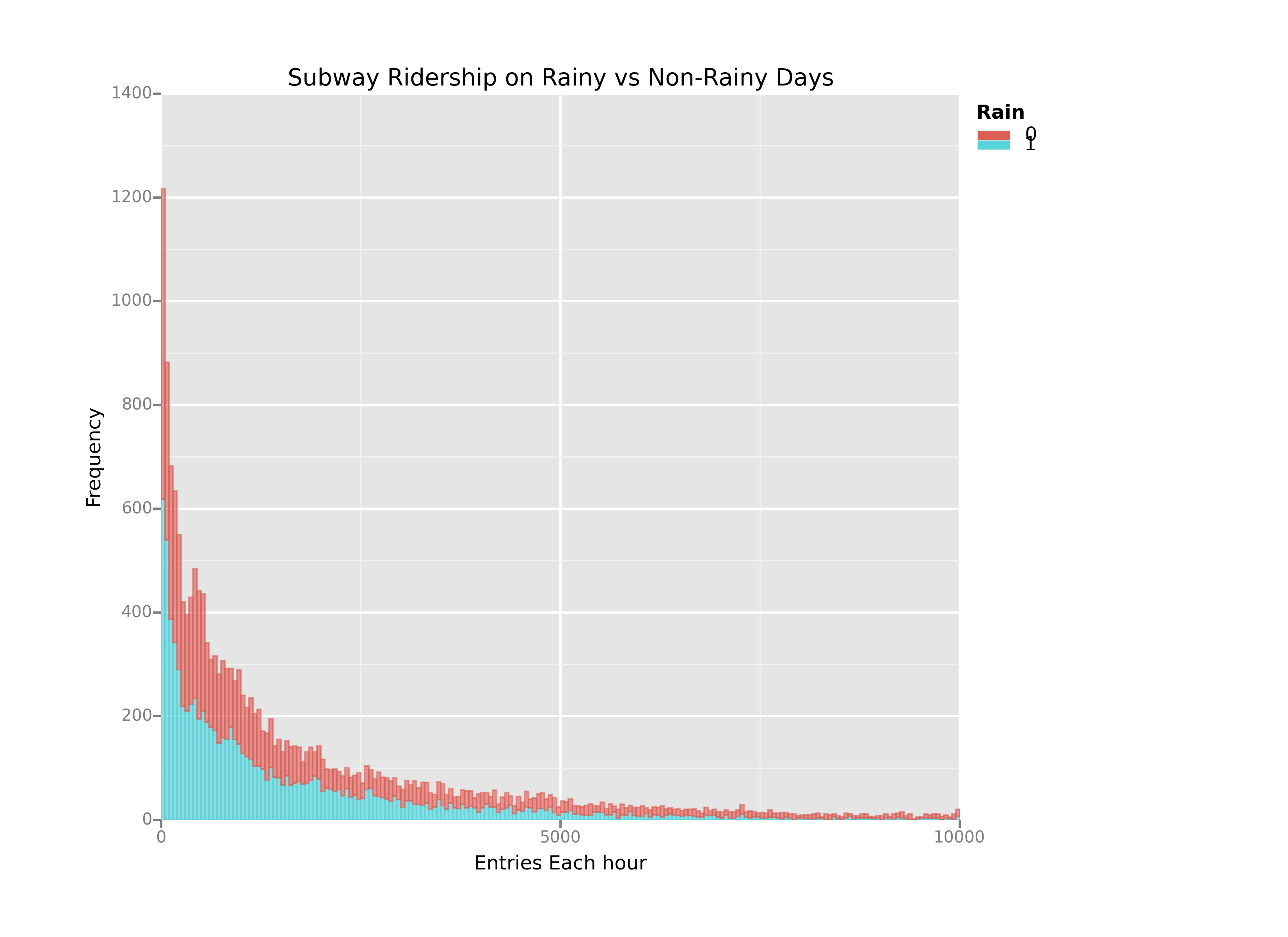
It may look like that the entries for the rainy day are more than the rainy days but this is false interpretation available from the graph. The graph looks like because the number of entries of the non-rainy days is much more than number of entries for rainy days.
3.2 Visualization for Rider ship by time of day.
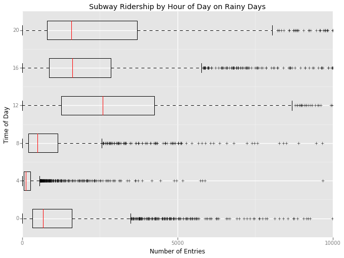
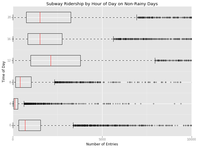
From the visualization is section 3.2 it is clear that number of entries for the subway increase at 12 pm and 8 pm. But this may due to the aggregation of entries in 4 hour slots. Also the boxes (IQR) for the 12pm and 20pm are bigger on rainy days than on non rainy days.
Section 4 : Conclusion
4.1 From the analysis of the data it can be interpreted that more people ride the NYC subway when it is raining than when it is not raining.
4.2 The above analysis can be concluded as of following reasons
The samples of the people riding when it’s raining and when it’s not raining are statistically different and relevant as given by the p-value. Since the mean value of ridership during rain is more hence we can say that more people ride in the subway while it’s raining outside.
Nothing can be conclusively said by the parameters of the linear regression model but the coefficient value of the rain parameter in the model is positive and significant with respect to other parameters taken. Hence it is evident that raining outside has positive effect on the subway ridership.
Section 5 : Reflection
5.1 Shortcomings of the method and analysis
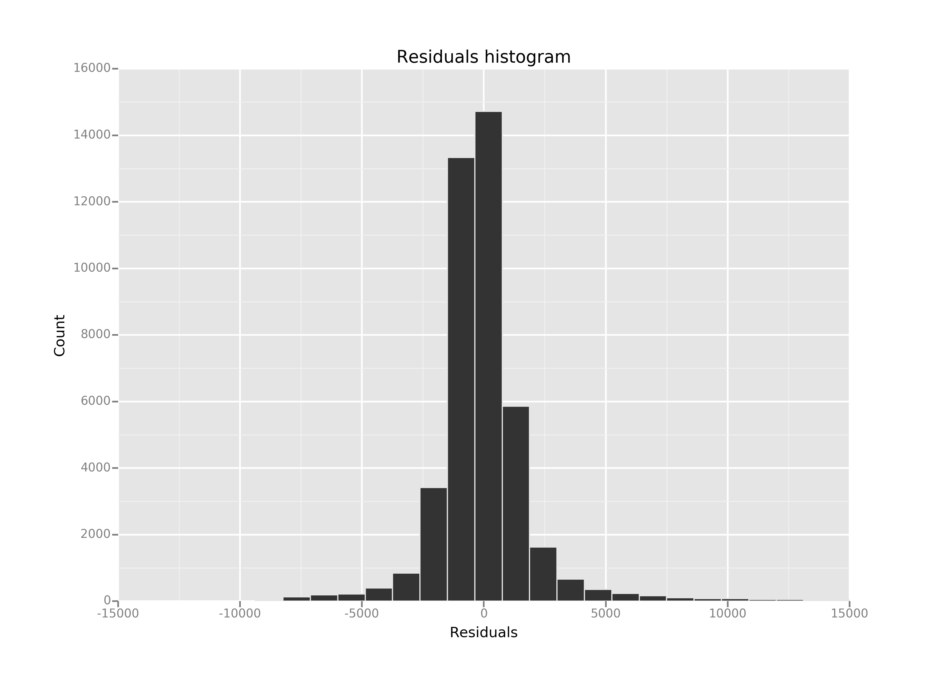
This dataset is good for basic analysis of the ridership and learning of the concepts but since the data is only of the May 2011 then this will only give us information of ridership according to month which may be dependent upon other factors. Also the data of hourly entries is I think clubbed into the interval of 4 hours. This generalization may also give false information about ridership at particular hour. Linear regression is a basic tool to get the feel of the data and if the data can be linearly modelled then it is a good tool but in the event of non-linear relationships, it may not provide the best analysis. I have used the ordinary least squares model for the model generation but there are other models also with different cost functions that may provide a better model. As for the features that I have taken as input are minimal (only 3) as of adding more features the R-squared value was increasing but that was not practically significant to make the model more complex. The residual plot has some long tails which calls for need of more exploration and may be different transformations of the data.
In the end, this project gave a good overview of the process of taking a dataset and do some analysis on it.