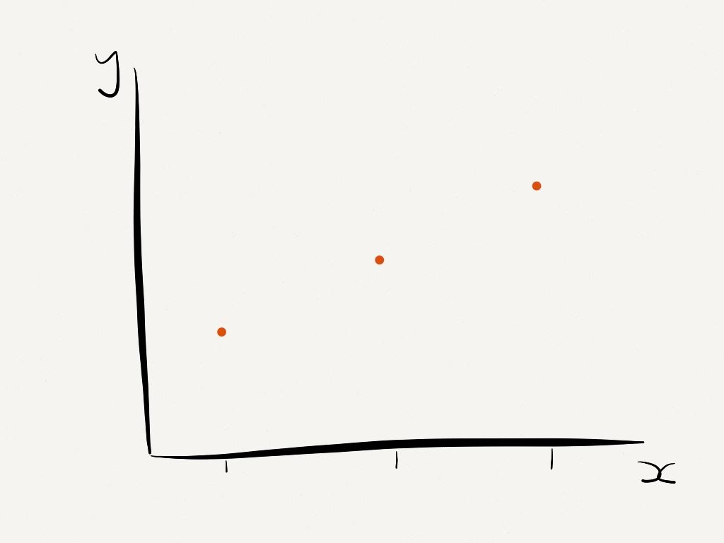
We can start by thinking of time series analysis as a regression problem, with
\[ y(x) = f(x) + \epsilon\]
Where \(y(x)\) is the output of interest, \(f(x)\) is some function and \(\epsilon\) is an additive white noise process.
We would like to:
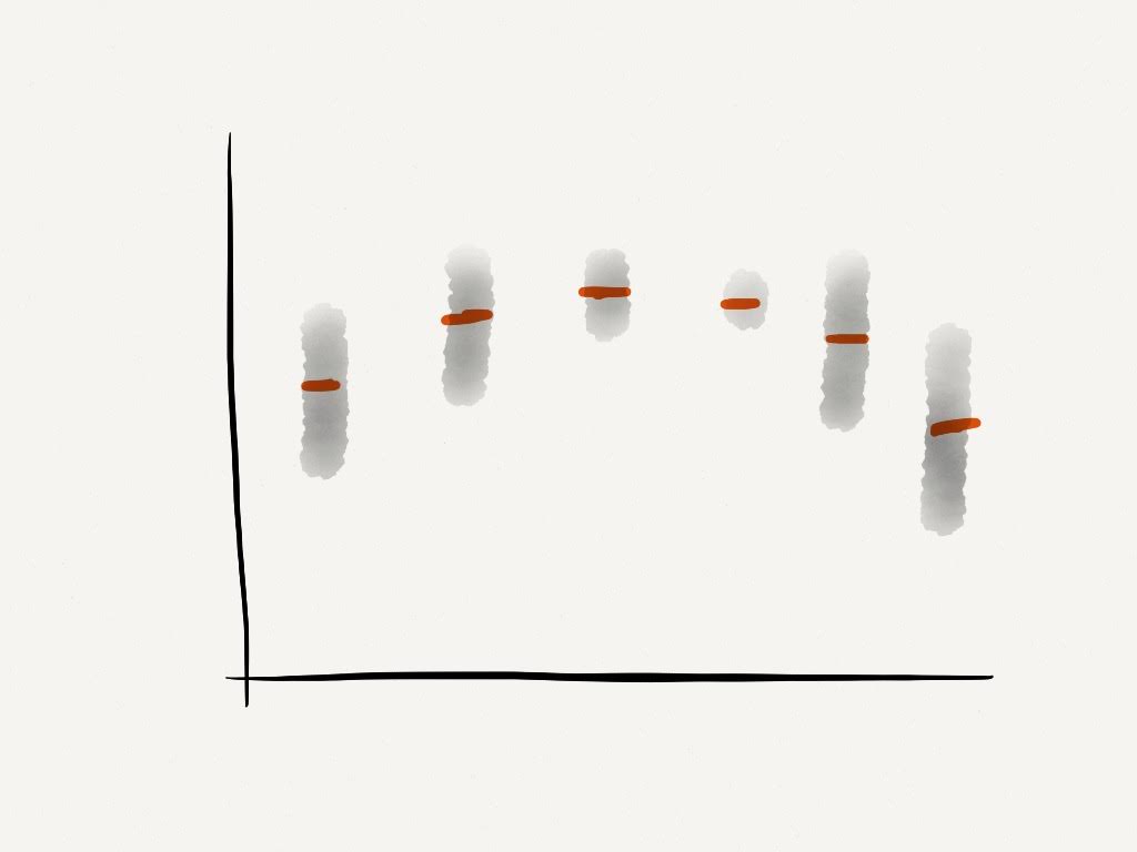
- Evaluate \(f(x)\)
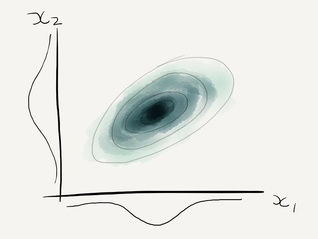
- Find the probability distribution of \(y^*\) for some \(x^*\)
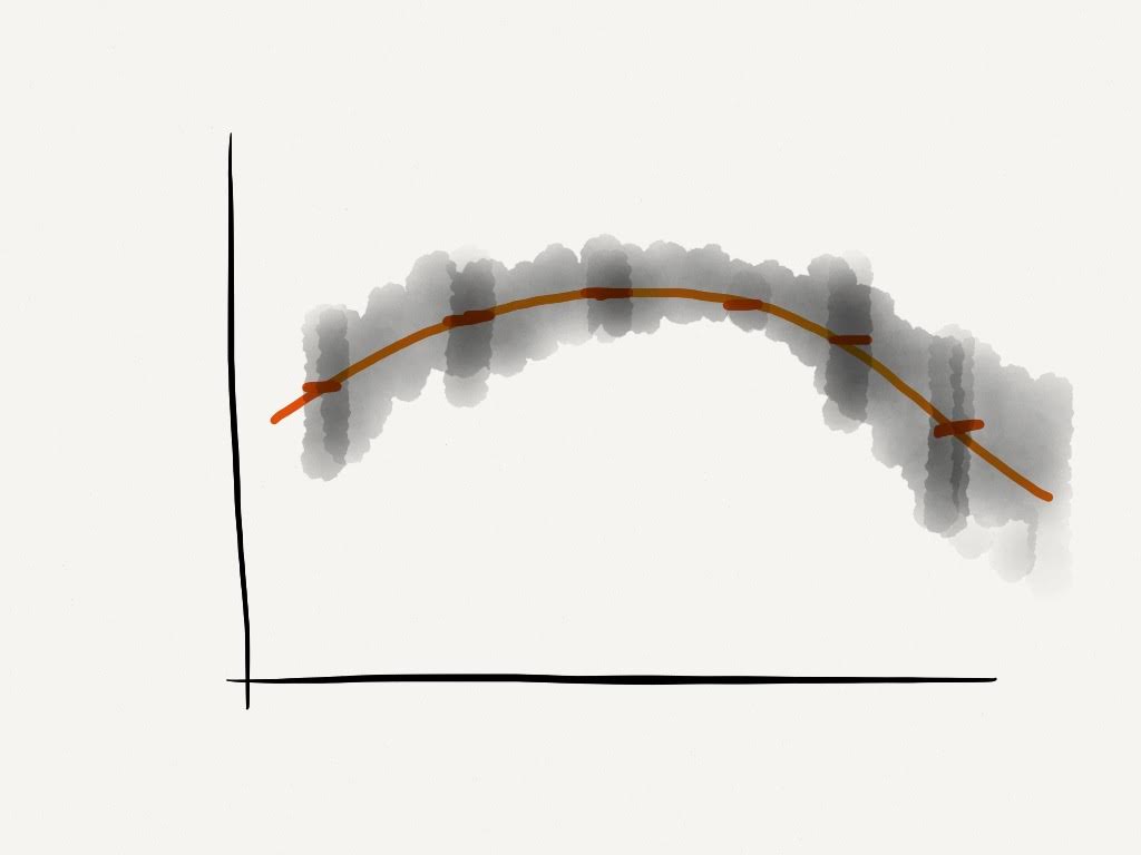
We make the assumption that \(y\) is ordered by \(x\), we fit a curve to the points and extrapolate.