Learning outcomes

In this lecture we will:

  • Learn some key time series concepts and features
  • Get to see some of the example time series that we'll use on the course
  • Understand the types of analysis that we want to do, and why
  • Learn to avoid some common mistakes

What is a time series?

  • A collection of data indexed by (strictly increasing) time
  • Can be regular or irregular
  • Usually one value per time

“With one dimension marching along to the regular rhythm of seconds, minutes, hours, days, weeks, months, years, centuries, or millennia, the natural ordering of the time scale gives this design a strength and efficiency of interpretation found in no other graphic arrangement.”

Edward R. TufteThe Visual Display of Quantitative Informationp. 28
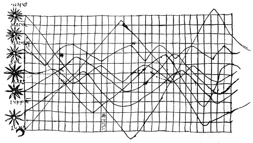
The first time series example?

Skipping forward a bit …

Diagram showing the distance of the planets to the earth in 1732, also showing a complete lunar eclipse and a partial solar eclipse in that yearNicolaas Kruik 1678 - 1754 Dutch Astronomer & Meteorologist

Lambert

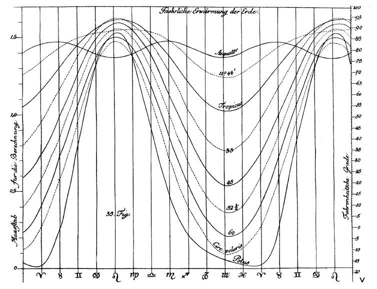
A graph of solar warming vs. lattitude.
Johann Heinrich Lambert 1728 - 1777

Application to economic data

Willaim Playfair's trade-balance time-series chart, published in his Commercial and Political Atlas, 1786

Time Series Analysis: What's the point?

What do we use time series methods for? Often, we are trying to do at least one of the following:

  1. Description: what is going on?
  2. Understanding: how is it going on, and why?
  3. Prediction: What is going to go on next?

First, description

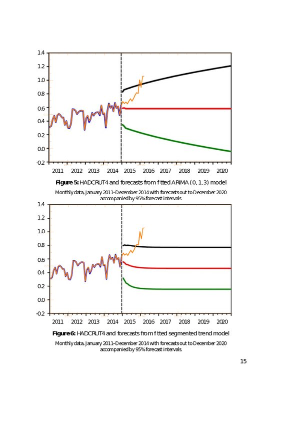
  • HadCRUT4 Annual globally averaged surface temperature, from the Met Office Hadley Centre and Climate Research Unit, UEA.

  • How do we separate the structure (here the long term trend) and the random noise?

Plot the data

  • Using a line plot gives a slightly different impression.

What is going on?

We get a different impression again if we just plot the last 15 years …

What is going on?

So, what is structure?

And what is random?

And, how does that randomness manifest?

A simpler example? Sea level rise

  • Church and White
  • There appears relatively less noise in this data compared to the trend

How do we go about it?

We know there is randomness and uncertainty in the time series. We can use a statistical model to help us understand and predict the system. This usually proceeds:

  1. Model identification and selection
  2. Parameter estimation
  3. Model checking

There are a number of features of time series and concepts that help in the process …

Time series features & concepts

Periodicity and cycles

  • Time series may show periodicity and cycles - often seasonal, but perhaps with more complexity.
plot(ldeaths)

Changes in variability & Heteroskedasticity

  • This AirPassengers data set shows heteroskedasticity - changes in variability.
plot(AirPassengers)

Example - GISP2 stable isotope ratios in Greenland ice

  • This data shows heteroskedacity and regime changes and a lot of structure

Autocorrelation and memory

  • Autocorrelation is the correlation of a random process with itself at a different time.

Smoothing

  • When we smooth a time series, we are applying a filter to try and remove some of the randomness, and get at (or remove) the underlying structure.
  • We are making assumptions, and imposing structure. You have to put something in in order to get something out.

Stationarity

  • In a stationary time series mean, variance and autocorrelation structure do not change over time.
  • Stationarity is a common assumption in some types of time series analysis.

Differencing

  • A time series of the differences between the values.
  • Differencing can be used used to make a non-stationary trend stationary.
  • First differencing removes a linear trend, \(k\)th-order differencing removes a polynomial trend of order \(k\)

The limits of our analysis

The Lynx data

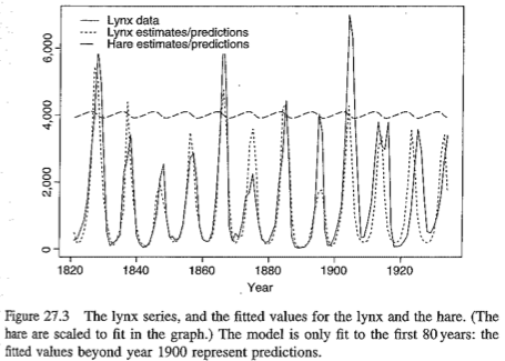
This is the lynx data set, annual numbers of lynx trappings for Canada 1821 - 1934. Regarded as representative of the population.

plot(lynx)

The Lynx data

Forecasting is hard

"Prediction is very difficult, especially about the future" - Niels Bohr

(Graphic from D. Spiegelhalter)

Forecasting is hard

Forecasting is hard

In summary

This course takes a practical approach, and should help you:

  • Understand modern Bayesian modelling techniques.
  • Get and use tools for thinking about and dealing with uncertainty.
  • Fit time series models, and make predictions.
  • Understand your time series data, and the process that generates it.