Be the boss of your factors
- Load the Gapminder data
- Model life expectancy as a function of year
- Get to know the country factor
- Why the order of factor levels matters
droplevels()to drop unused factor levelsreorder()to reorder factor levelsreorder()exercise- Revaluing factor levels
- Grow a factor object
- Make a factor from scratch
As of 2016-10-11 this is deprecated. STAT 545 is now using the forcats package for factor management, which is covered in the current factor lesson.
Load the Gapminder data
As usual, load the Gapminder excerpt and the ggplot2 package. Load plyr and/or dplyr. If you load both, load plyr first.
library(gapminder)
library(plyr)
suppressPackageStartupMessages(library(dplyr))
library(ggplot2)
Model life expectancy as a function of year
For each country, retain estimated intercept and slope from a linear fit – regressing life expectancy on year. First, we write a function that does the work for one country.
le_lin_fit <- function(dat, offset = 1952) {
  the_fit <- lm(lifeExp ~ I(year - offset), dat)
  setNames(data.frame(t(coef(the_fit))), c("intercept", "slope"))
}
gapminder %>%
  filter(country == "Canada") %>%
  le_lin_fit()
##   intercept     slope
## 1  68.88385 0.2188692
Now we split the data up by country and apply this function. In both approaches, we include country AND continent in the factors on which to split, so both appear in the result.
First, the dplyr way:
gcoefs <- gapminder %>%
  group_by(country, continent) %>%
  do(le_lin_fit(.)) %>%
  ungroup()
gcoefs
## # A tibble: 142 × 4
##        country continent intercept     slope
##         <fctr>    <fctr>     <dbl>     <dbl>
## 1  Afghanistan      Asia  29.90729 0.2753287
## 2      Albania    Europe  59.22913 0.3346832
## 3      Algeria    Africa  43.37497 0.5692797
## 4       Angola    Africa  32.12665 0.2093399
## 5    Argentina  Americas  62.68844 0.2317084
## 6    Australia   Oceania  68.40051 0.2277238
## 7      Austria    Europe  66.44846 0.2419923
## 8      Bahrain      Asia  52.74921 0.4675077
## 9   Bangladesh      Asia  36.13549 0.4981308
## 10     Belgium    Europe  67.89192 0.2090846
## # ... with 132 more rows
Or, if you wish, the plyr way:
gcoefs2 <- ddply(gapminder, ~ country + continent, le_lin_fit)
gcoefs2
##                      country continent intercept       slope
## 1                Afghanistan      Asia  29.90729  0.27532867
## 2                    Albania    Europe  59.22913  0.33468322
## 3                    Algeria    Africa  43.37497  0.56927972
## 4                     Angola    Africa  32.12665  0.20933986
## 5                  Argentina  Americas  62.68844  0.23170839
## 6                  Australia   Oceania  68.40051  0.22772378
## 7                    Austria    Europe  66.44846  0.24199231
## 8                    Bahrain      Asia  52.74921  0.46750769
## 9                 Bangladesh      Asia  36.13549  0.49813077
## 10                   Belgium    Europe  67.89192  0.20908462
## 11                     Benin    Africa  39.58851  0.33423287
## 12                   Bolivia  Americas  38.75645  0.49993217
## 13    Bosnia and Herzegovina    Europe  58.08956  0.34975524
## 14                  Botswana    Africa  52.92912  0.06066853
## 15                    Brazil  Americas  51.51204  0.39008951
## 16                  Bulgaria    Europe  65.73731  0.14568881
## 17              Burkina Faso    Africa  34.68469  0.36397483
## 18                   Burundi    Africa  40.57864  0.15413427
## 19                  Cambodia      Asia  37.01542  0.39590280
## 20                  Cameroon    Africa  41.24946  0.25014685
## 21                    Canada  Americas  68.88385  0.21886923
## 22  Central African Republic    Africa  38.80951  0.18390559
## 23                      Chad    Africa  39.80937  0.25324406
## 24                     Chile  Americas  54.31771  0.47684406
## 25                     China      Asia  47.19048  0.53071485
## 26                  Colombia  Americas  53.42712  0.38075035
## 27                   Comoros    Africa  39.99600  0.45039091
## 28          Congo, Dem. Rep.    Africa  41.96108  0.09391538
## 29               Congo, Rep.    Africa  47.13678  0.19509580
## 30                Costa Rica  Americas  59.10471  0.40278951
## 31             Cote d'Ivoire    Africa  44.84586  0.13055664
## 32                   Croatia    Europe  63.85578  0.22545944
## 33                      Cuba  Americas  62.21345  0.32115035
## 34            Czech Republic    Europe  67.52808  0.14481538
## 35                   Denmark    Europe  71.03359  0.12133007
## 36                  Djibouti    Africa  36.27715  0.36740350
## 37        Dominican Republic  Americas  48.59781  0.47115245
## 38                   Ecuador  Americas  49.06537  0.50005315
## 39                     Egypt    Africa  40.96800  0.55545455
## 40               El Salvador  Americas  46.51195  0.47714126
## 41         Equatorial Guinea    Africa  34.43031  0.31017063
## 42                   Eritrea    Africa  35.69527  0.37469021
## 43                  Ethiopia    Africa  36.02815  0.30718531
## 44                   Finland    Europe  66.44897  0.23792517
## 45                    France    Europe  67.79013  0.23850140
## 46                     Gabon    Africa  38.93535  0.44673287
## 47                    Gambia    Africa  28.40037  0.58182587
## 48                   Germany    Europe  67.56813  0.21368322
## 49                     Ghana    Africa  43.49274  0.32174266
## 50                    Greece    Europe  67.06721  0.24239860
## 51                 Guatemala  Americas  42.11940  0.53127343
## 52                    Guinea    Africa  31.55699  0.42483077
## 53             Guinea-Bissau    Africa  31.73704  0.27175315
## 54                     Haiti  Americas  39.24615  0.39705804
## 55                  Honduras  Americas  42.99241  0.54285175
## 56          Hong Kong, China      Asia  63.42864  0.36597063
## 57                   Hungary    Europe  65.99282  0.12364895
## 58                   Iceland    Europe  71.96359  0.16537552
## 59                     India      Asia  39.26976  0.50532098
## 60                 Indonesia      Asia  36.88312  0.63464126
## 61                      Iran      Asia  44.97899  0.49663986
## 62                      Iraq      Asia  50.11346  0.23521049
## 63                   Ireland    Europe  67.54146  0.19911958
## 64                    Israel      Asia  66.30041  0.26710629
## 65                     Italy    Europe  66.59679  0.26971049
## 66                   Jamaica  Americas  62.66099  0.22139441
## 67                     Japan      Asia  65.12205  0.35290420
## 68                    Jordan      Asia  44.06386  0.57172937
## 69                     Kenya    Africa  47.00204  0.20650769
## 70          Korea, Dem. Rep.      Asia  54.90560  0.31642657
## 71               Korea, Rep.      Asia  49.72750  0.55540000
## 72                    Kuwait      Asia  57.45933  0.41683636
## 73                   Lebanon      Asia  58.68736  0.26102937
## 74                   Lesotho    Africa  47.37903  0.09556573
## 75                   Liberia    Africa  39.83642  0.09599371
## 76                     Libya    Africa  42.10194  0.62553566
## 77                Madagascar    Africa  36.66806  0.40372797
## 78                    Malawi    Africa  36.91037  0.23422587
## 79                  Malaysia      Asia  51.50522  0.46452238
## 80                      Mali    Africa  33.05123  0.37680979
## 81                Mauritania    Africa  40.02560  0.44641748
## 82                 Mauritius    Africa  55.37077  0.34845385
## 83                    Mexico  Americas  53.00537  0.45103497
## 84                  Mongolia      Asia  43.82641  0.43868811
## 85                Montenegro    Europe  62.24163  0.29300140
## 86                   Morocco    Africa  42.69083  0.54247273
## 87                Mozambique    Africa  34.20615  0.22448531
## 88                   Myanmar      Asia  41.41155  0.43309510
## 89                   Namibia    Africa  47.13433  0.23116364
## 90                     Nepal      Asia  34.43164  0.52926154
## 91               Netherlands    Europe  71.88962  0.13668671
## 92               New Zealand   Oceania  68.68692  0.19282098
## 93                 Nicaragua  Americas  43.04513  0.55651958
## 94                     Niger    Africa  35.15067  0.34210909
## 95                   Nigeria    Africa  37.85953  0.20806573
## 96                    Norway    Europe  72.21462  0.13194126
## 97                      Oman      Asia  37.20774  0.77217902
## 98                  Pakistan      Asia  43.72296  0.40579231
## 99                    Panama  Americas  58.06100  0.35420909
## 100                 Paraguay  Americas  62.48183  0.15735455
## 101                     Peru  Americas  44.34764  0.52769790
## 102              Philippines      Asia  49.40435  0.42046923
## 103                   Poland    Europe  64.78090  0.19621888
## 104                 Portugal    Europe  61.14679  0.33720140
## 105              Puerto Rico  Americas  66.94853  0.21057483
## 106                  Reunion    Africa  53.99754  0.45988042
## 107                  Romania    Europe  63.96213  0.15740140
## 108                   Rwanda    Africa  42.74195 -0.04583147
## 109    Sao Tome and Principe    Africa  48.52756  0.34068252
## 110             Saudi Arabia      Asia  40.81412  0.64962308
## 111                  Senegal    Africa  36.74667  0.50470000
## 112                   Serbia    Europe  61.53435  0.25515105
## 113             Sierra Leone    Africa  30.88321  0.21403497
## 114                Singapore      Asia  61.84588  0.34088601
## 115          Slovak Republic    Europe  67.00987  0.13404406
## 116                 Slovenia    Europe  66.08635  0.20052378
## 117                  Somalia    Africa  34.67540  0.22957343
## 118             South Africa    Africa  49.34128  0.16915944
## 119                    Spain    Europe  66.47782  0.28093077
## 120                Sri Lanka      Asia  59.79149  0.24489441
## 121                    Sudan    Africa  37.87419  0.38277483
## 122                Swaziland    Africa  46.38786  0.09507483
## 123                   Sweden    Europe  71.60500  0.16625455
## 124              Switzerland    Europe  69.45372  0.22223147
## 125                    Syria      Asia  46.10128  0.55435944
## 126                   Taiwan      Asia  61.33744  0.32724476
## 127                 Tanzania    Africa  43.10841  0.17468811
## 128                 Thailand      Asia  52.65642  0.34704825
## 129                     Togo    Africa  40.97746  0.38259231
## 130      Trinidad and Tobago  Americas  62.05231  0.17366154
## 131                  Tunisia    Africa  44.55531  0.58784336
## 132                   Turkey    Europe  46.02232  0.49723986
## 133                   Uganda    Africa  44.27522  0.12158601
## 134           United Kingdom    Europe  68.80853  0.18596573
## 135            United States  Americas  68.41385  0.18416923
## 136                  Uruguay  Americas  65.74160  0.18327203
## 137                Venezuela  Americas  57.51332  0.32972168
## 138                  Vietnam      Asia  39.01008  0.67161538
## 139       West Bank and Gaza      Asia  43.79840  0.60110070
## 140              Yemen, Rep.      Asia  30.13028  0.60545944
## 141                   Zambia    Africa  47.65803 -0.06042517
## 142                 Zimbabwe    Africa  55.22124 -0.09302098
all.equal(gcoefs, gcoefs2)
## [1] TRUE
Get to know the country factor
str(gcoefs, give.attr = FALSE)
## Classes 'tbl_df', 'tbl' and 'data.frame':    142 obs. of  4 variables:
##  $ country  : Factor w/ 142 levels "Afghanistan",..: 1 2 3 4 5 6 7 8 9 10 ...
##  $ continent: Factor w/ 5 levels "Africa","Americas",..: 3 4 1 1 2 5 4 3 3 4 ...
##  $ intercept: num  29.9 59.2 43.4 32.1 62.7 ...
##  $ slope    : num  0.275 0.335 0.569 0.209 0.232 ...
levels(gcoefs$country)
##   [1] "Afghanistan"              "Albania"
##   [3] "Algeria"                  "Angola"
##   [5] "Argentina"                "Australia"
##   [7] "Austria"                  "Bahrain"
##   [9] "Bangladesh"               "Belgium"
##  [11] "Benin"                    "Bolivia"
##  [13] "Bosnia and Herzegovina"   "Botswana"
##  [15] "Brazil"                   "Bulgaria"
##  [17] "Burkina Faso"             "Burundi"
##  [19] "Cambodia"                 "Cameroon"
##  [21] "Canada"                   "Central African Republic"
##  [23] "Chad"                     "Chile"
##  [25] "China"                    "Colombia"
##  [27] "Comoros"                  "Congo, Dem. Rep."
##  [29] "Congo, Rep."              "Costa Rica"
##  [31] "Cote d'Ivoire"            "Croatia"
##  [33] "Cuba"                     "Czech Republic"
##  [35] "Denmark"                  "Djibouti"
##  [37] "Dominican Republic"       "Ecuador"
##  [39] "Egypt"                    "El Salvador"
##  [41] "Equatorial Guinea"        "Eritrea"
##  [43] "Ethiopia"                 "Finland"
##  [45] "France"                   "Gabon"
##  [47] "Gambia"                   "Germany"
##  [49] "Ghana"                    "Greece"
##  [51] "Guatemala"                "Guinea"
##  [53] "Guinea-Bissau"            "Haiti"
##  [55] "Honduras"                 "Hong Kong, China"
##  [57] "Hungary"                  "Iceland"
##  [59] "India"                    "Indonesia"
##  [61] "Iran"                     "Iraq"
##  [63] "Ireland"                  "Israel"
##  [65] "Italy"                    "Jamaica"
##  [67] "Japan"                    "Jordan"
##  [69] "Kenya"                    "Korea, Dem. Rep."
##  [71] "Korea, Rep."              "Kuwait"
##  [73] "Lebanon"                  "Lesotho"
##  [75] "Liberia"                  "Libya"
##  [77] "Madagascar"               "Malawi"
##  [79] "Malaysia"                 "Mali"
##  [81] "Mauritania"               "Mauritius"
##  [83] "Mexico"                   "Mongolia"
##  [85] "Montenegro"               "Morocco"
##  [87] "Mozambique"               "Myanmar"
##  [89] "Namibia"                  "Nepal"
##  [91] "Netherlands"              "New Zealand"
##  [93] "Nicaragua"                "Niger"
##  [95] "Nigeria"                  "Norway"
##  [97] "Oman"                     "Pakistan"
##  [99] "Panama"                   "Paraguay"
## [101] "Peru"                     "Philippines"
## [103] "Poland"                   "Portugal"
## [105] "Puerto Rico"              "Reunion"
## [107] "Romania"                  "Rwanda"
## [109] "Sao Tome and Principe"    "Saudi Arabia"
## [111] "Senegal"                  "Serbia"
## [113] "Sierra Leone"             "Singapore"
## [115] "Slovak Republic"          "Slovenia"
## [117] "Somalia"                  "South Africa"
## [119] "Spain"                    "Sri Lanka"
## [121] "Sudan"                    "Swaziland"
## [123] "Sweden"                   "Switzerland"
## [125] "Syria"                    "Taiwan"
## [127] "Tanzania"                 "Thailand"
## [129] "Togo"                     "Trinidad and Tobago"
## [131] "Tunisia"                  "Turkey"
## [133] "Uganda"                   "United Kingdom"
## [135] "United States"            "Uruguay"
## [137] "Venezuela"                "Vietnam"
## [139] "West Bank and Gaza"       "Yemen, Rep."
## [141] "Zambia"                   "Zimbabwe"
head(gcoefs$country)
## [1] Afghanistan Albania     Algeria     Angola      Argentina   Australia
## 142 Levels: Afghanistan Albania Algeria Angola Argentina ... Zimbabwe
The levels are in alphabetical order. Why? Because. Just because. Do you have a better idea? THEN STEP UP AND DO SOMETHING ABOUT IT.
Why the order of factor levels matters
ggplot(gcoefs, aes(x = slope, y = country)) + geom_point()
ggplot(gcoefs, aes(x = slope, y = reorder(country, slope))) +
  geom_point()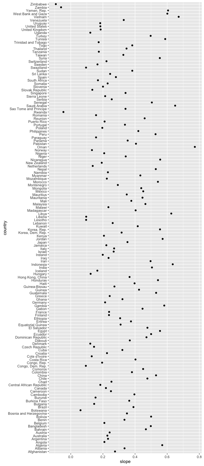
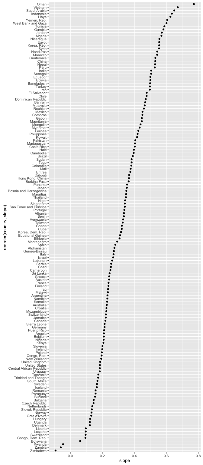
Which figure do you find easier to navigate? Which is more interesting? The unsorted, i.e. alphabetical, is an example of visual data puke, because there is no effort to help the viewer learn anything from the plot, even though it is really easy to do so. At the very least, always consider sorting your factor levels in some principled way.
The same point generally applies to tables as well.
Exercise (part of HW05): Consider post_arrange, post_reorder, and post_both as defined below. State how the objects differ and discuss the differences in terms of utility within an exploratory analysis. If I swapped out arrange(country) for arrange(slope), would we get the same result? Do you have any preference for one arrange statement over the other?
post_arrange <- gcoefs %>% arrange(slope)
post_reorder <- gcoefs %>%
  mutate(country = reorder(country, slope))
post_both <- gcoefs %>%
  mutate(country = reorder(country, slope)) %>%
  arrange(country)
droplevels() to drop unused factor levels
Many demos will be clearer if we create a smaller dataset with just a few countries.
Let’s look at these five countries: Egypt, Haiti, Romania, Thailand, Venezuela.
h_countries <- c("Egypt", "Haiti", "Romania", "Thailand", "Venezuela")
hDat <- gapminder %>%
  filter(country %in% h_countries)
hDat %>% str()
## Classes 'tbl_df', 'tbl' and 'data.frame':    60 obs. of  6 variables:
##  $ country  : Factor w/ 142 levels "Afghanistan",..: 39 39 39 39 39 39 39 39 39 39 ...
##  $ continent: Factor w/ 5 levels "Africa","Americas",..: 1 1 1 1 1 1 1 1 1 1 ...
##  $ year     : int  1952 1957 1962 1967 1972 1977 1982 1987 1992 1997 ...
##  $ lifeExp  : num  41.9 44.4 47 49.3 51.1 ...
##  $ pop      : int  22223309 25009741 28173309 31681188 34807417 38783863 45681811 52799062 59402198 66134291 ...
##  $ gdpPercap: num  1419 1459 1693 1815 2024 ...
Look at the country factor. Look at it hard.
#table(hDat$country)
#levels(hDat$country)
nlevels(hDat$country)
## [1] 142
Even though hDat contains data for only 5 countries, the other 137 countries remain as possible levels of the country factor. Sometimes this is exactly what you want but sometimes it’s not.
When you want to drop unused factor levels, use droplevels().
iDat  <- hDat %>% droplevels()
iDat %>% str()
## Classes 'tbl_df', 'tbl' and 'data.frame':    60 obs. of  6 variables:
##  $ country  : Factor w/ 5 levels "Egypt","Haiti",..: 1 1 1 1 1 1 1 1 1 1 ...
##  $ continent: Factor w/ 4 levels "Africa","Americas",..: 1 1 1 1 1 1 1 1 1 1 ...
##  $ year     : int  1952 1957 1962 1967 1972 1977 1982 1987 1992 1997 ...
##  $ lifeExp  : num  41.9 44.4 47 49.3 51.1 ...
##  $ pop      : int  22223309 25009741 28173309 31681188 34807417 38783863 45681811 52799062 59402198 66134291 ...
##  $ gdpPercap: num  1419 1459 1693 1815 2024 ...
table(iDat$country)
##
##     Egypt     Haiti   Romania  Thailand Venezuela
##        12        12        12        12        12
levels(iDat$country)
## [1] "Egypt"     "Haiti"     "Romania"   "Thailand"  "Venezuela"
nlevels(iDat$country)
## [1] 5
reorder() to reorder factor levels
Now that we have a more manageable set of 5 countries, let’s compute their max life expectancies, view them, and view life expectancy vs. year.
i_le_max <- iDat %>%
  group_by(country) %>%
  summarize(max_le = max(lifeExp))
i_le_max
## # A tibble: 5 × 2
##     country max_le
##      <fctr>  <dbl>
## 1     Egypt 71.338
## 2     Haiti 60.916
## 3   Romania 72.476
## 4  Thailand 70.616
## 5 Venezuela 73.747
ggplot(i_le_max, aes(x = country, y = max_le, group = 1)) +
geom_path() + geom_point()
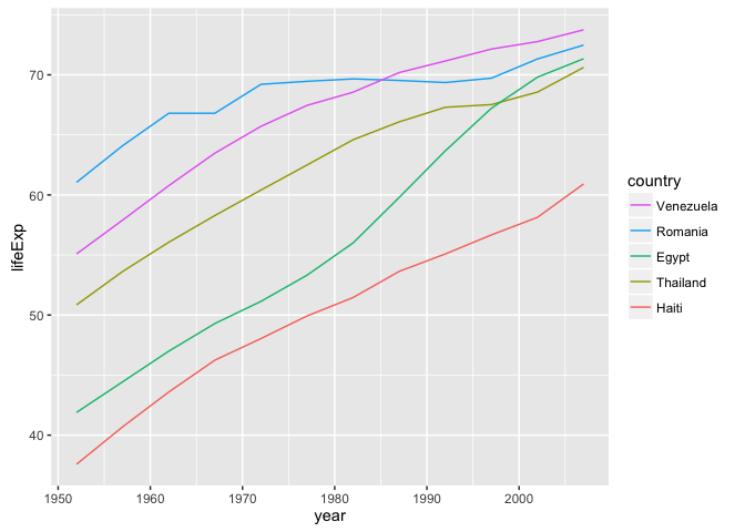
ggplot(iDat, aes(x = year, y = lifeExp, group = country)) +
geom_line(aes(color = country))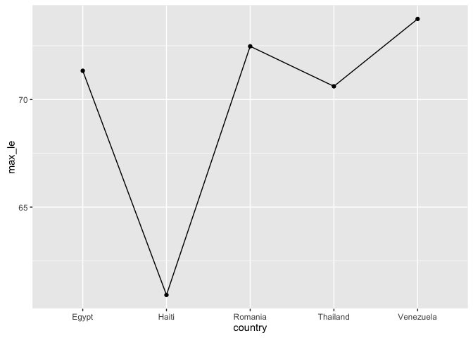
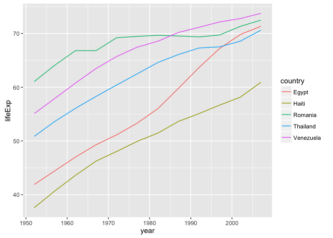
Here’s a plot of the max life expectancies and a spaghetti plot of life expectancy over time. Notice how the first plot jumps around? Notice how the legend of the second plot is completely out of order with the data?
Use the function reorder() to change the order of factor levels. Read its documentation.
reorder(your_factor, your_quant_var, your_summarization_function)Let’s reorder the country factor logically, in this case by maximum life expectancy. Even though i_le_max already holds these numbers, I’m going to enact the reordering with the “raw” data to illustrate more about the reorder() function.
jDat <- iDat %>%
  mutate(country = reorder(country, lifeExp, max))
data.frame(before = levels(iDat$country), after = levels(jDat$country))
##      before     after
## 1     Egypt     Haiti
## 2     Haiti  Thailand
## 3   Romania     Egypt
## 4  Thailand   Romania
## 5 Venezuela Venezuela
j_le_max <- i_le_max %>%
  mutate(country = reorder(country, max_le))
j_le_max <- i_le_max %>%
  mutate(country = factor(country, levels = levels(jDat$country)))
Let’s revisit the two figures to see how much more natural they are.
ggplot(j_le_max, aes(x = country, y = max_le, group = 1)) +
  geom_line() + geom_point()
ggplot(jDat, aes(x = year, y = lifeExp)) +
  geom_line(aes(color = country)) +
  guides(color = guide_legend(reverse = TRUE))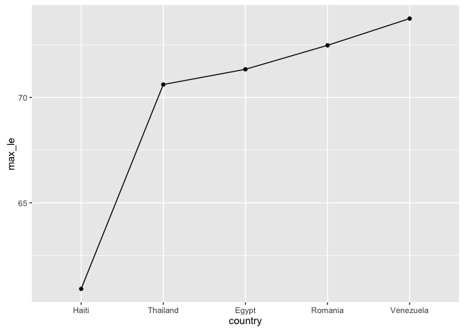
Conclusion: Use reorder() to reorder a factor according to a quantitative variable. A simple call like this:
reorder(your_factor, your_quant_var)implies that the summarization function will default to mean(). If that’s not what you want, specify your own summarization function. It could be built-in, such as max(), or could be written by you on-the-fly or in advance.
You can do this and alter your actual data (or a new copy thereof). Or you can do this reordering on-the-fly, i.e. in an actual plotting or tabulation call, leaving the underlying data untouched.
reorder() exercise
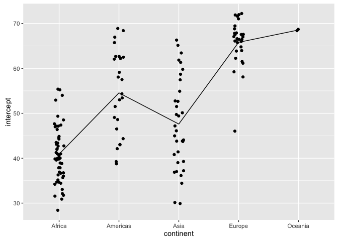
Reorder the continent factor, according to the estimated intercepts.
To review, remember we have computed the estimated intercept and slope for each country:
head(gcoefs)
## # A tibble: 6 × 4
##       country continent intercept     slope
##        <fctr>    <fctr>     <dbl>     <dbl>
## 1 Afghanistan      Asia  29.90729 0.2753287
## 2     Albania    Europe  59.22913 0.3346832
## 3     Algeria    Africa  43.37497 0.5692797
## 4      Angola    Africa  32.12665 0.2093399
## 5   Argentina  Americas  62.68844 0.2317084
## 6   Australia   Oceania  68.40051 0.2277238
The figure on the left gives a stripplot of estimate intercepts, by continent, with continent in alphabetical order. The line connects continent-specific averages of the intercepts (approx. equal to life expectancy in 1952). The figure on the right gives same plot after the continents have been reordered by average estimated intercept.
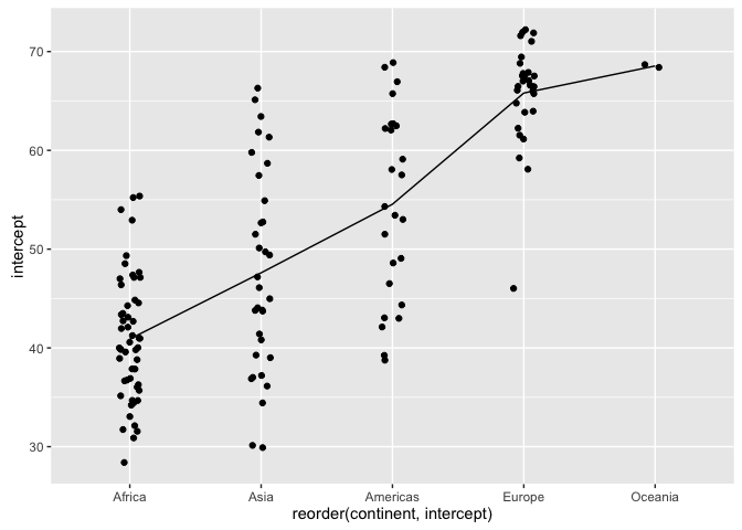
Exercise: Write the reorder() statement to do this.
Revaluing factor levels
What if you want to recode factor levels? I usually use the revalue() function from plyr; sometime I use plyr::mapvalues() which is a bit more general. In the past I have also used the recode() function from the car package.
k_countries <- c("Australia", "Korea, Dem. Rep.", "Korea, Rep.")
kDat <- gapminder %>%
  filter(country %in% k_countries, year > 2000) %>%
  droplevels()
kDat
## # A tibble: 6 × 6
##            country continent  year lifeExp      pop gdpPercap
##             <fctr>    <fctr> <int>   <dbl>    <int>     <dbl>
## 1        Australia   Oceania  2002  80.370 19546792 30687.755
## 2        Australia   Oceania  2007  81.235 20434176 34435.367
## 3 Korea, Dem. Rep.      Asia  2002  66.662 22215365  1646.758
## 4 Korea, Dem. Rep.      Asia  2007  67.297 23301725  1593.065
## 5      Korea, Rep.      Asia  2002  77.045 47969150 19233.988
## 6      Korea, Rep.      Asia  2007  78.623 49044790 23348.140
levels(kDat$country)
## [1] "Australia"        "Korea, Dem. Rep." "Korea, Rep."
kDat <- kDat %>%
  mutate(new_country = revalue(country,
                               c("Australia" = "Oz",
                                 "Korea, Dem. Rep." = "North Korea",
                                 "Korea, Rep." = "South Korea")))
data_frame(levels(kDat$country), levels(kDat$new_country))
## # A tibble: 3 × 2
##   `levels(kDat$country)` `levels(kDat$new_country)`
##                    <chr>                      <chr>
## 1              Australia                         Oz
## 2       Korea, Dem. Rep.                North Korea
## 3            Korea, Rep.                South Korea
kDat
## # A tibble: 6 × 7
##            country continent  year lifeExp      pop gdpPercap new_country
##             <fctr>    <fctr> <int>   <dbl>    <int>     <dbl>      <fctr>
## 1        Australia   Oceania  2002  80.370 19546792 30687.755          Oz
## 2        Australia   Oceania  2007  81.235 20434176 34435.367          Oz
## 3 Korea, Dem. Rep.      Asia  2002  66.662 22215365  1646.758 North Korea
## 4 Korea, Dem. Rep.      Asia  2007  67.297 23301725  1593.065 North Korea
## 5      Korea, Rep.      Asia  2002  77.045 47969150 19233.988 South Korea
## 6      Korea, Rep.      Asia  2007  78.623 49044790 23348.140 South Korea
Grow a factor object
Try to avoid this. If you must rbind()ing data.frames works much better than c()ing vectors.
usa <- gapminder %>%
  filter(country == "United States", year > 2000) %>%
  droplevels()
mex <- gapminder %>%
  filter(country == "Mexico", year > 2000) %>%
  droplevels()
str(usa)
## Classes 'tbl_df', 'tbl' and 'data.frame':    2 obs. of  6 variables:
##  $ country  : Factor w/ 1 level "United States": 1 1
##  $ continent: Factor w/ 1 level "Americas": 1 1
##  $ year     : int  2002 2007
##  $ lifeExp  : num  77.3 78.2
##  $ pop      : int  287675526 301139947
##  $ gdpPercap: num  39097 42952
str(mex)
## Classes 'tbl_df', 'tbl' and 'data.frame':    2 obs. of  6 variables:
##  $ country  : Factor w/ 1 level "Mexico": 1 1
##  $ continent: Factor w/ 1 level "Americas": 1 1
##  $ year     : int  2002 2007
##  $ lifeExp  : num  74.9 76.2
##  $ pop      : int  102479927 108700891
##  $ gdpPercap: num  10742 11978
usa_mex <- rbind(usa, mex)
## rbinding data.frames works!
str(usa_mex)
## Classes 'tbl_df', 'tbl' and 'data.frame':    4 obs. of  6 variables:
##  $ country  : Factor w/ 2 levels "United States",..: 1 1 2 2
##  $ continent: Factor w/ 1 level "Americas": 1 1 1 1
##  $ year     : int  2002 2007 2002 2007
##  $ lifeExp  : num  77.3 78.2 74.9 76.2
##  $ pop      : int  287675526 301139947 102479927 108700891
##  $ gdpPercap: num  39097 42952 10742 11978

## simply catenating factors does not work!
(oops <- c(usa$country, mex$country))
## [1] 1 1 1 1

## workaround
(yeah <- factor(c(levels(usa$country)[usa$country],
                  levels(mex$country)[mex$country])))
## [1] United States United States Mexico        Mexico
## Levels: Mexico United States
If you really want to catenate factors with different levels, you must first convert to their levels as character data, combine, then re-convert to factor.
Make a factor from scratch
The factor() function will explicitly create a factor de novo. Let’s start with an example we are familiar with. Pretend the continent variable in gapminder was a not a factor, but character.
gapminder$continent <- as.character(gapminder$continent)

#prove it
str(gapminder)
## Classes 'tbl_df', 'tbl' and 'data.frame':    1704 obs. of  6 variables:
##  $ country  : Factor w/ 142 levels "Afghanistan",..: 1 1 1 1 1 1 1 1 1 1 ...
##  $ continent: chr  "Asia" "Asia" "Asia" "Asia" ...
##  $ year     : int  1952 1957 1962 1967 1972 1977 1982 1987 1992 1997 ...
##  $ lifeExp  : num  28.8 30.3 32 34 36.1 ...
##  $ pop      : int  8425333 9240934 10267083 11537966 13079460 14880372 12881816 13867957 16317921 22227415 ...
##  $ gdpPercap: num  779 821 853 836 740 ...
head(gapminder)
## # A tibble: 6 × 6
##       country continent  year lifeExp      pop gdpPercap
##        <fctr>     <chr> <int>   <dbl>    <int>     <dbl>
## 1 Afghanistan      Asia  1952  28.801  8425333  779.4453
## 2 Afghanistan      Asia  1957  30.332  9240934  820.8530
## 3 Afghanistan      Asia  1962  31.997 10267083  853.1007
## 4 Afghanistan      Asia  1967  34.020 11537966  836.1971
## 5 Afghanistan      Asia  1972  36.088 13079460  739.9811
## 6 Afghanistan      Asia  1977  38.438 14880372  786.1134
We can now turn it back into a factor by calling factor. The first argument is the input (usually character), followed by factor levels, which will default to the unique input values, in alphabetical order.
gapminder$continent <- factor(gapminder$continent)

#prove it
str(gapminder)
## Classes 'tbl_df', 'tbl' and 'data.frame':    1704 obs. of  6 variables:
##  $ country  : Factor w/ 142 levels "Afghanistan",..: 1 1 1 1 1 1 1 1 1 1 ...
##  $ continent: Factor w/ 5 levels "Africa","Americas",..: 3 3 3 3 3 3 3 3 3 3 ...
##  $ year     : int  1952 1957 1962 1967 1972 1977 1982 1987 1992 1997 ...
##  $ lifeExp  : num  28.8 30.3 32 34 36.1 ...
##  $ pop      : int  8425333 9240934 10267083 11537966 13079460 14880372 12881816 13867957 16317921 22227415 ...
##  $ gdpPercap: num  779 821 853 836 740 ...
head(gapminder)
## # A tibble: 6 × 6
##       country continent  year lifeExp      pop gdpPercap
##        <fctr>    <fctr> <int>   <dbl>    <int>     <dbl>
## 1 Afghanistan      Asia  1952  28.801  8425333  779.4453
## 2 Afghanistan      Asia  1957  30.332  9240934  820.8530
## 3 Afghanistan      Asia  1962  31.997 10267083  853.1007
## 4 Afghanistan      Asia  1967  34.020 11537966  836.1971
## 5 Afghanistan      Asia  1972  36.088 13079460  739.9811
## 6 Afghanistan      Asia  1977  38.438 14880372  786.1134