kolzur_filter module¶

Version : 2017-03-31

Summary¶

Functions¶

`_kz_coeffs`(m, k)	Calculate coefficients of the Kolmogorov–Zurbenko filter
`_kz_prod`(data, coef, m, k[, t])
`_kz_sum`(data, coef)
`kz_filter`(data, m, k)	Kolmogorov-Zurbenko fitler
`kzft`(data, nu, m, k[, t, dt])	Kolmogorov-Zurbenko Fourier transform filter
`kzp`(data, nu, m, k[, dt])	Kolmogorov-Zurbenko periodogram
`sliding_window`(arr, window)	Apply a sliding window on a numpy array.

Introduction¶

Numpy implementation of the Kolmogorov-Zurbenko filter

https://en.wikipedia.org/wiki/Kolmogorov%E2%80%93Zurbenko_filter

Todo

Implement the KZ adaptive filter.

Functions¶

_kz_coeffs(m, k)[source]¶

Calculate coefficients of the Kolmogorov–Zurbenko filter

Returns:	A `numpy.ndarray` of size k*(m-1)+1

This functions returns the normlalised coefficients $a_s^{m,k}/m^k$ .

Coefficients definition

A definition of the Kolmogorov–Zurbenko filter coefficients is provided in this article. Coefficients $a_s^{m,k}$ are the coefficients of the polynomial function: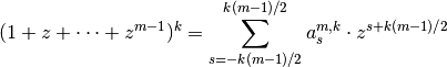

$(1 + z + \cdots + z^{m-1})^k = \sum_{s=-k(m-1)/2}^{k(m-1)/2} a_s^{m,k} \cdot z^{s+k(m-1)/2}$

The $a_s^{m,k}$ coefficients are calculated by iterating over $k$ .

Calculation example for m=5 and k=3

Let us define the polynomial function

$P(z) = 1 + z + z^2 + z^3 + z^4.$

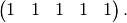
At $k=1$ , the coefficients $a_s^{m,k}=a_s^{1,5}$ are that of $P(z)$ ,

$\left(\begin{matrix} 1 & 1 & 1 & 1 & 1 \end{matrix}\right).$

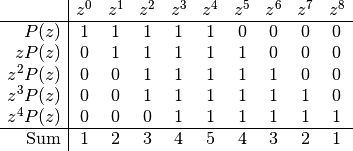
At $k=2$ , we want to calculate the coefficients of polynomial function $P(z)\cdot P(z)$ , of degree 8. First, we calculate the polynomial functions $P(z)$ , $zP(z)$ , $z^2P(z)$ and $z^3P(z)$ and then sum them.

Let us represent the coefficients of these functions in a table, with monomial elements in columns:

$\begin{array}{r|ccccccccc} & z^0 & z^1 & z^2 & z^3 & z^4 & z^5 & z^6 & z^7 & z^8 \\ \hline P(z) & 1 & 1 & 1 & 1 & 1 & 0 & 0 & 0 & 0 \\ zP(z) & 0 & 1 & 1 & 1 & 1 & 1 & 0 & 0 & 0 \\ z^2P(z) & 0 & 0 & 1 & 1 & 1 & 1 & 1 & 0 & 0 \\ z^3P(z) & 0 & 0 & 1 & 1 & 1 & 1 & 1 & 1 & 0 \\ z^4P(z) & 0 & 0 & 0 & 1 & 1 & 1 & 1 & 1 & 1 \\ \hline \mathrm{Sum} & 1 & 2 & 3 & 4 & 5 & 4 & 3 & 2 & 1 \end{array}$

At $k=3$ , we want to calculate the coefficients of polynomial function $P(z)\cdot P(z)^2$ , of degree 12. We use the same representation:

$\begin{array}{r|ccccccccccccc} & z^0 & z^1 & z^2 & z^3 & z^4 & z^5 & z^6 & z^7 & z^8 & z^9 & z^{10} & z^{11} & z^{12} \\ \hline P(z)^2 & 1 & 2 & 3 & 4 & 5 & 4 & 3 & 2 & 1 & 0 & 0 & 0 & 0 \\ zP(z)^2 & 0 & 1 & 2 & 3 & 4 & 5 & 4 & 3 & 2 & 1 & 0 & 0 & 0 \\ z^2P(z)^2 & 0 & 0 & 1 & 2 & 3 & 4 & 5 & 4 & 3 & 2 & 1 & 0 & 0 \\ z^3P(z)^2 & 0 & 0 & 0 & 1 & 2 & 3 & 4 & 5 & 4 & 3 & 2 & 1 & 0 \\ z^4P(z)^2 & 0 & 0 & 0 & 0 & 1 & 2 & 3 & 4 & 5 & 4 & 3 & 2 & 1 \\ \hline \mathrm{Sum} & 1 & 3 & 6 & 10 & 15 & 18 & 19 & 18 & 15 & 10 & 6 & 3 & 1 \end{array}$

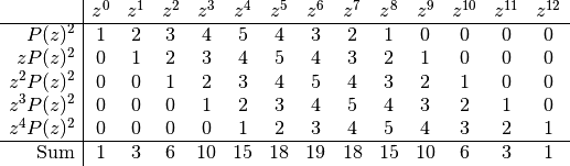
>>> c = _kz_coeffs(3, 1)
>>> print(c)
[ 0.33333333  0.33333333  0.33333333]
>>> c = _kz_coeffs(3, 2)
>>> print(c*3**2)
[ 1.  2.  3.  2.  1.]
>>> c = _kz_coeffs(5, 3)
>>> print(c*5**3)
[  1.   3.   6.  10.  15.  18.  19.  18.  15.  10.   6.   3.   1.]

_kz_prod(data, coef, m, k, t=None)[source]¶

_kz_sum(data, coef)[source]¶

kz_filter(data, m, k)[source]¶

Kolmogorov-Zurbenko fitler

Parameters:	data (numpy.ndarray) – A 1-dimensional numpy array of size N. Any missing value should be set to `np.nan`. m (int) – Filter window width. k (int) – Filter degree.
Returns:	A `numpy.ndarray` of size N-k*(m-1)

Given a time series $X_t, t \in \{0, 1, \cdots, N-1\}$ , the Kolmogorov-Zurbenko fitler is defined for $t \in \{\frac{k(m-1)}{2}, \cdots, N-1-\frac{k(m-1)}{2}\}$ by

$KZ_{m,k}[X_t] = \sum_{s=-k(m-1)/2}^{k(m-1)/2} \frac{a_s^{m,k}}{m^k} \cdot X_{t+s}$

Definition of coefficients $a_s^{m,k}$ is given in _kz_coeffs().

kzft(data, nu, m, k, t=None, dt=1.0)[source]¶

Kolmogorov-Zurbenko Fourier transform filter

Parameters:	data (numpy.ndarray) – A 1-dimensional numpy array of size N. Any missing value should be set to `np.nan`. nu (list-like) – Frequencies, length Nnu. m (int) – Filter window width. k (int) – Filter degree. t (list-like) – Calculation indices, of length Nt. If provided, KZFT filter will be calculated only for values `data[t]`. Note that the KZFT filter can only be calculated for indices in the range [k(m-1)/2, (N-1)-k(m-1)/2]. Trying to calculate the KZFT out of this range will raise an IndexError. None, calculation will happen over the whole calculable range. dt (float) – Time step, if not 1.
Returns:	A `numpy.ndarray` of shape (Nnu, Nt) or (Nnu, N-k(m-1)) if t is None.
Raises:	IndexError – If t contains one or more indices out of the calculation range. See documentation of keyword argument t.

Given a time series $X_t, t \in \{0, 1, \cdots, N-1\}$ , the Kolmogorov-Zurbenko Fourier transform filter is defined for $t \in \{\frac{k(m-1)}{2}, \cdots, N-1-\frac{k(m-1)}{2}\}$ by

$KZFT_{m,k,\nu}[X_t] = \sum_{s=-k(m-1)/2}^{k(m-1)/2} \frac{a_s^{m,k}}{m^k} \cdot X_{t+s} \cdot e^{-2\pi i\nu s}$

kzp(data, nu, m, k, dt=1.0)[source]¶

Kolmogorov-Zurbenko periodogram

Parameters:	data (numpy.ndarray) – A 1-dimensional numpy array of size N. Any missing value should be set to `np.nan`. nu (list-like) – Frequencies, length Nnu. m (int) – Filter window width. k (int) – Filter degree. dt (float) – Time step, if not 1.
Returns:	A `numpy.ndarray` os size Nnu.

Given a time series $X_t, t \in \{0, 1, \cdots, N-1\}$ , the Kolmogorov-Zurbenko periodogram is defined by

$KZP_{m,k}(\nu) = \sqrt{\sum_{h=0}^{T-1} \lvert 2 \cdot KZFT_{m,k,\nu}[X_{hL+k(m-1)/2}] \rvert ^2}$

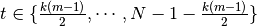
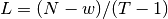where $L=(N-w)/(T-1)$ is the distance between the beginnings of two successive intervals, $w$ being the calculation window width of the kzft() and $T$ the number of intervals.

The assumption was made that $L \ll w \ll N$ , implying that the intervals overlap.

sliding_window(arr, window)[source]¶

Apply a sliding window on a numpy array.

Parameters:	arr (numpy.ndarray) – An array of shape (n1, ..., nN) window (int) – Window size.
Returns:	A `numpy.ndarray` of shape (n1, ..., nN-window+1, window).

Table Of Contents

This Page

kolzur_filter module¶

Summary¶

Functions¶

Introduction¶

Functions¶