This is a walkthrough of a simple 3-analysis example pipeline.
The goal of the pipeline is to multiply two long numbers. We pretend that it cannot be done in one operation on a single machine. So we decide to split the task into subtasks of multiplying the first long number by individual digits of the second long number for the sake of an example. At the last step the partial products are shifted and added together to yield the final product.
|
A J-diagram is a directed acyclic graph where nodes represent Jobs, Semaphores or Accumulators with edges representing relationships and dependencies. Most of these objects are created dynamically during the pipeline execution, so here you'll see a lot of action - the J-diagram will be growing. J-diagrams can be generated at any moment during a pipeline's execution by running Hive's visualize_jobs.pl script (new in version/2.5) . |
An A-diagram is a directed graph where most of the nodes represent Analyses and edges represent Rules. As a whole it represents the structure of the pipeline which is normally static. The only changing elements will be job counts and analysis colours. A-diagrams can be generated at any moment during a pipeline's execution by running Hive's generate_graph.pl script. |
The main bulk of this document is a commented series of snapshots of both types of diagrams during the execution of the pipeline.
They can be approximately reproduced by running a sequence of commands, similar to these, in a terminal:
    export PIPELINE_URL=sqlite:///lg4_long_mult.sqlite                                                               # An SQLite file is enough to handle this pipeline

    init_pipeline.pl Bio::EnsEMBL::Hive::Examples::LongMult::PipeConfig::LongMult_conf -pipeline_url $PIPELINE_URL   # Initialize the pipeline database from a PipeConfig file

    runWorker.pl -url $PIPELINE_URL -job_id $JOB_ID                                                                  # Run a specific job - this allows you to force your own order of execution. Run a few of these

    beekeeper.pl -url $PIPELINE_URL -analyses_pattern $ANALYSIS_NAME -sync                                           # Force the system to recalculate job counts and determine states of analyses

    visualize_jobs.pl -url $PIPELINE_URL -out long_mult_jobs_${STEP_NUMBER}.png                                      # To make a J-diagram snapshot (it is convenient to have synchronized numbering)

    generate_graph.pl -url $PIPELINE_URL -out long_mult_analyses_${STEP_NUMBER}.png                                  # To make an A-diagram snapshot (it is convenient to have synchronized numbering)
|
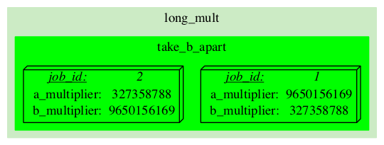
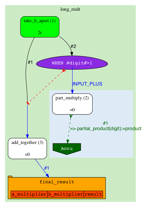
This is our pipeline just after the initialization:
|
|
|
The J-diagram shows a couple of 3d-boxes, they represent specific Jobs. Each Job is an individual task that can be run on an individual machine. We need at least one initial Job to run a pipeline. However that one Job may generate many more as it gets executed. In this example we have two initial Jobs. They were created automatically during the pipeline's initialization process. These two initial Jobs will generate two independent "streams" of execution which will yield their own independent results. Since in this particular pipeline we are simply multiplying same two numbers in different orders, we expect the final results to be identical. |
The A-diagram shows how execution of the pipeline is guided by Rules. Since the Rules are mostly static, the diagram will also be changing very little. The main objects on A-diagram are rectangles with rounded corners, they represent Analyses. Analyses are "types" of Jobs (Analyses broadly define which code to run, where and how, but miss specific parameters which become defined in Jobs). In this pipeline we have three types: 'take_b_apart', 'part_multiply' and 'add_together'. The "take_b_apart" Analysis contains two Jobs, which are in 'READY' state (can be checked-out for execution). Our colour for 'READY' is green, so both the Analysis and the specific Jobs are shown in green. |
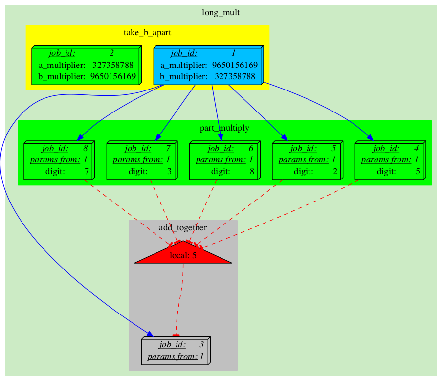
After running the first Job we see a lot of changes on the J-diagram:
|
|
|
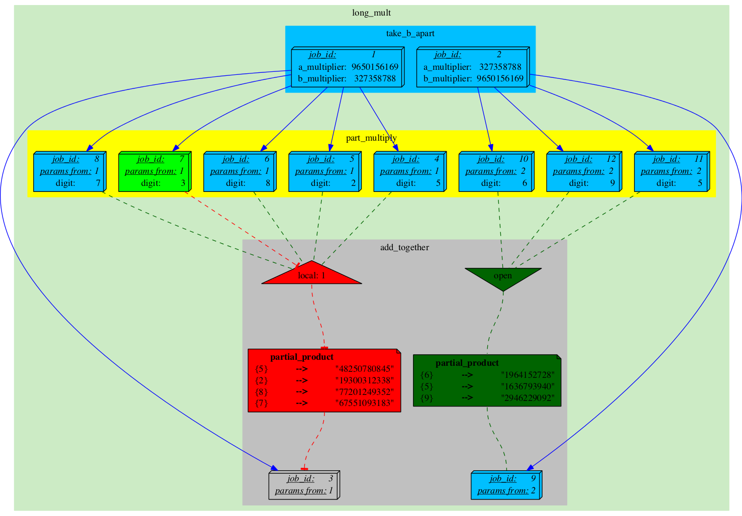
Job_1 has finished running and is now in 'DONE' state (colour-coded blue). It has generated 6 more Jobs: five in Analysis 'part_multiply' (splitting its own task into parts) and one in Analysis 'add_together' (which will recombine the results of the former into the final result). The newly created 'part_multiply' Jobs also control a Semaphore which blocks the 'add_together' Job which is in 'SEMAPHORED' state and cannot be executed yet (grey). The Semaphore is essentially a counter that gets decremented each time one of the controlling Jobs becomes 'DONE'. It is our primary mechanism for synchronization of control- and dataflow. |
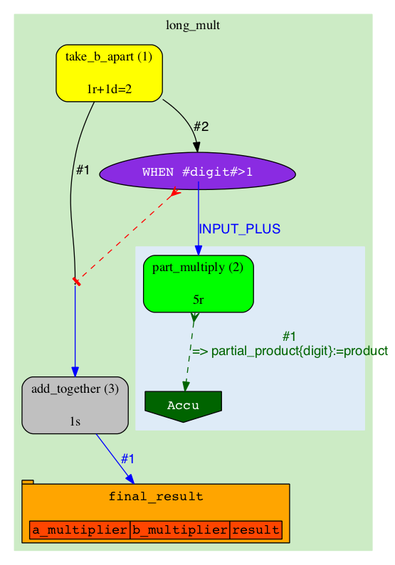
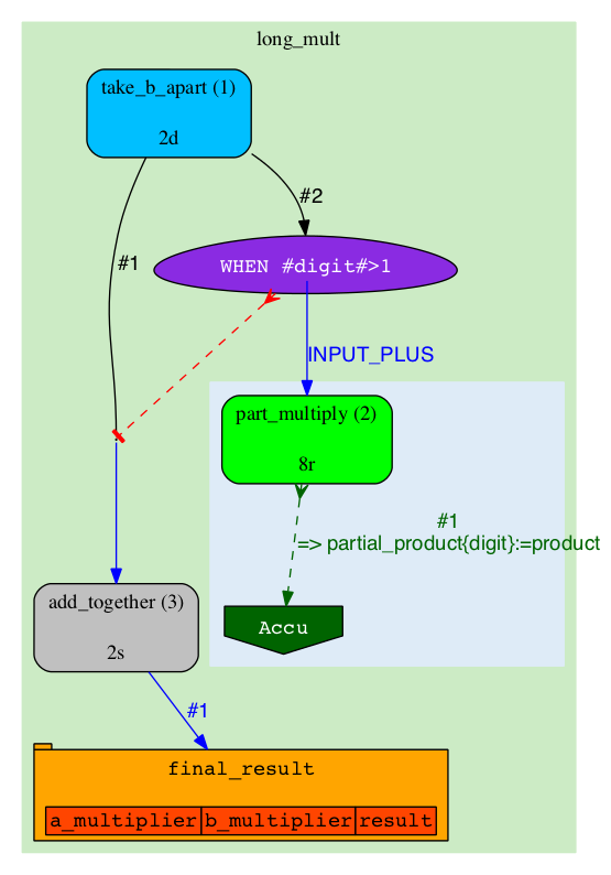
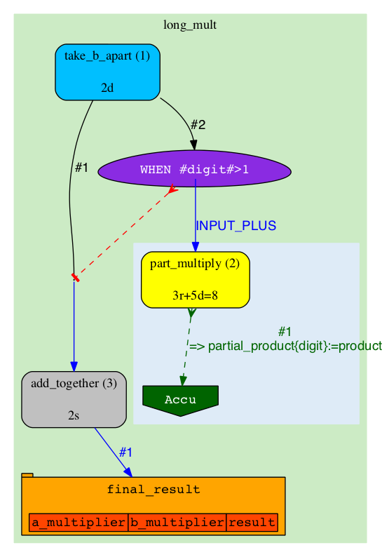
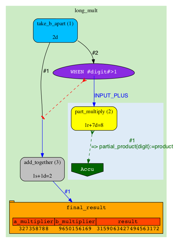
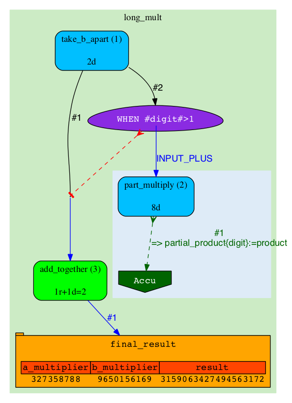
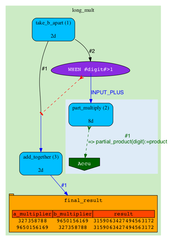
The topology of A-diagram doesn't normally change, so pay attention at more subtle changes of colours and labels:
|
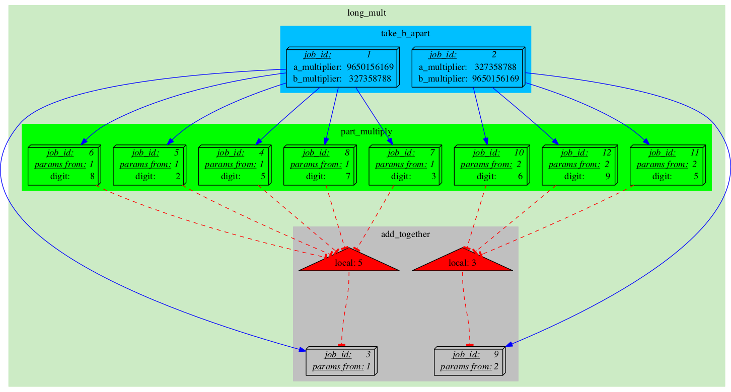
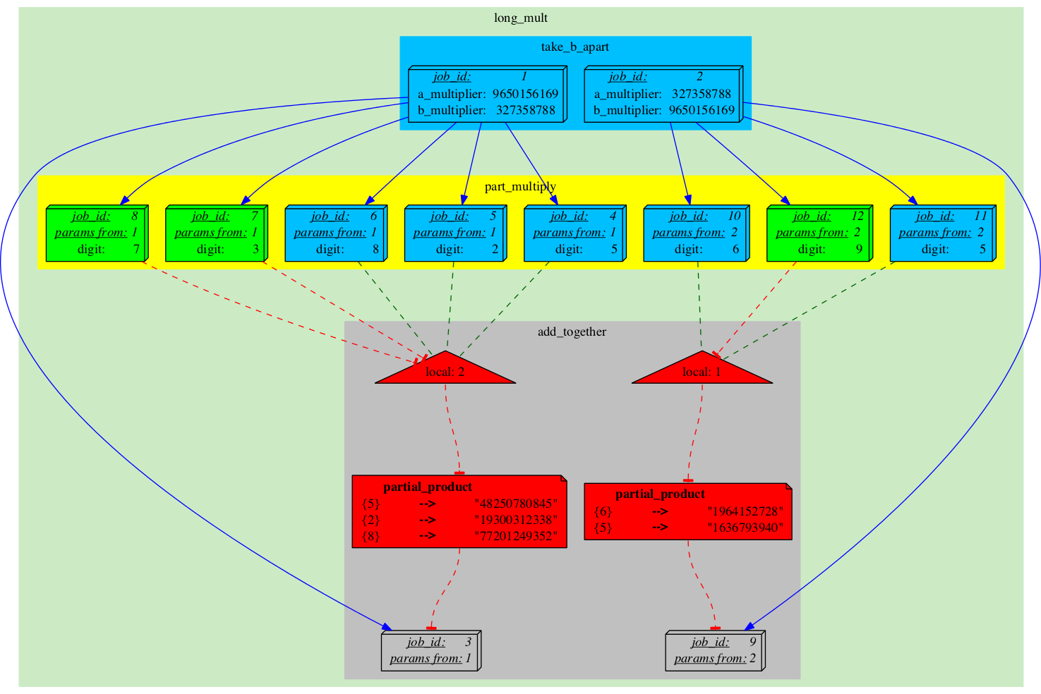
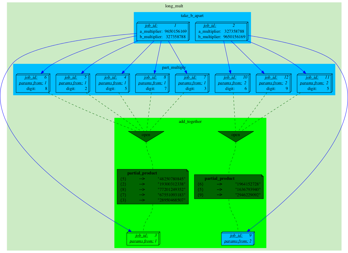
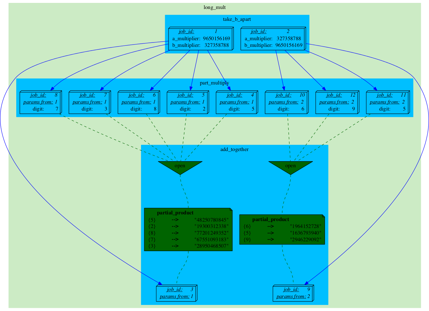
After running the second Job more jobs have been added to Analyses 'part_multiply' and 'add_together'.
|
|
|
There is a new Semaphore, a new group of 'part_multiply' Jobs to control it, and a new 'add_together' Job blocked by it. Note that the child jobs sometimes inherit some of their parameters from their parent Job ("params from: 1", "params from: 2"). This is done to save some space. |
|
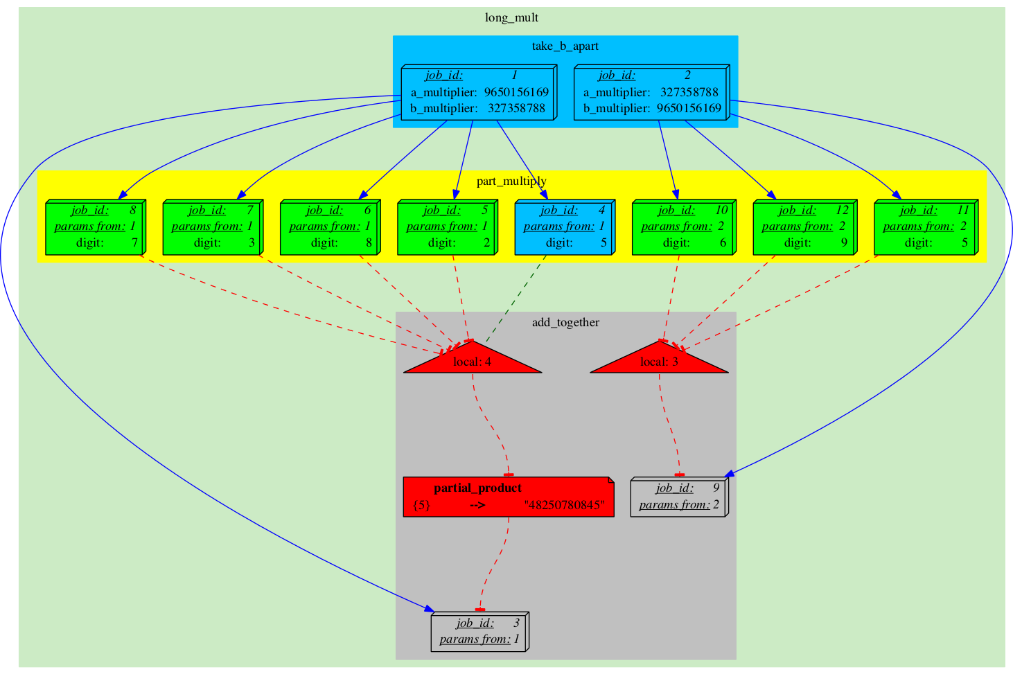
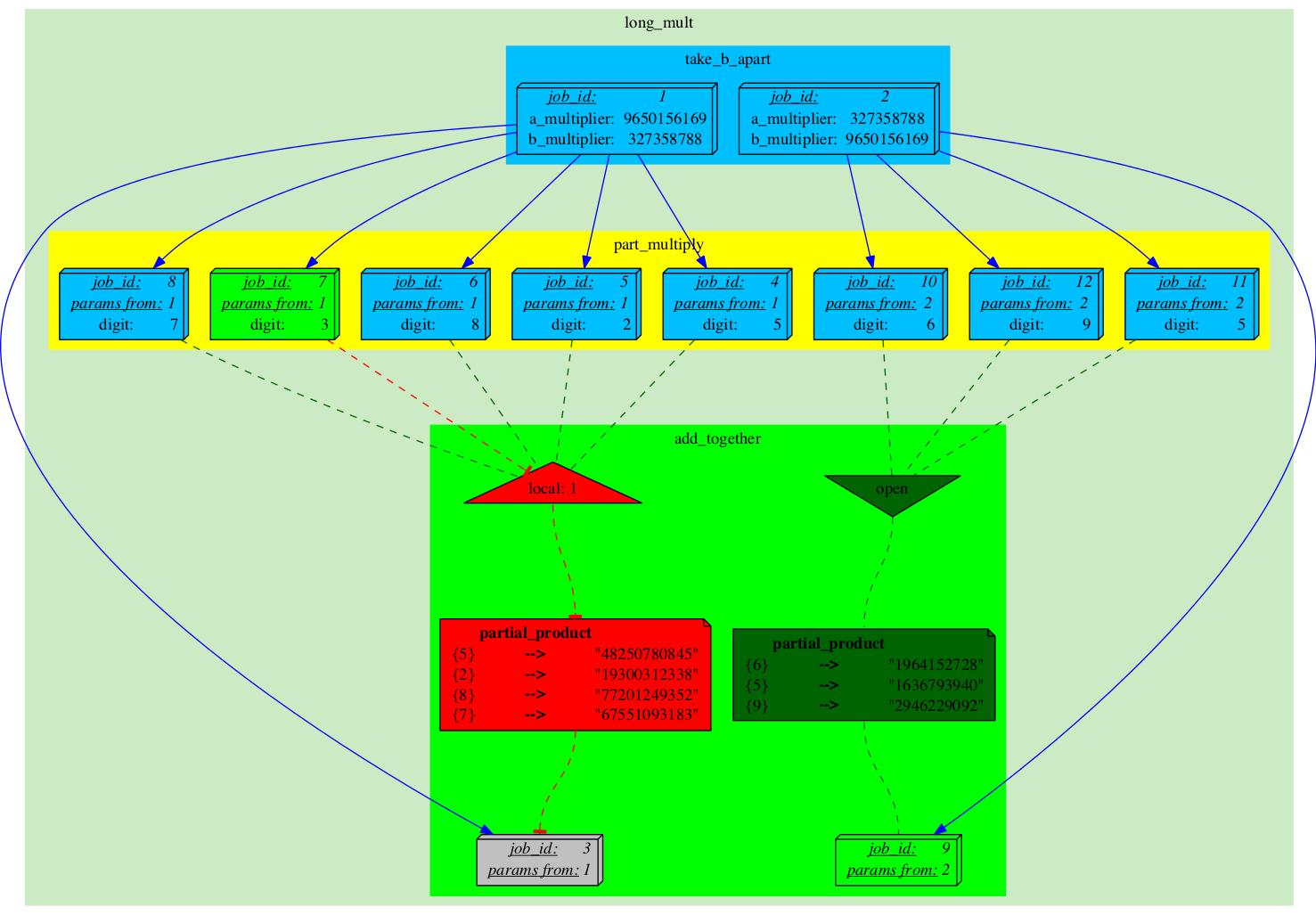
We finally get to run a Job from the second Analysis.
|

|
|
Once it's done, two things happen:
|
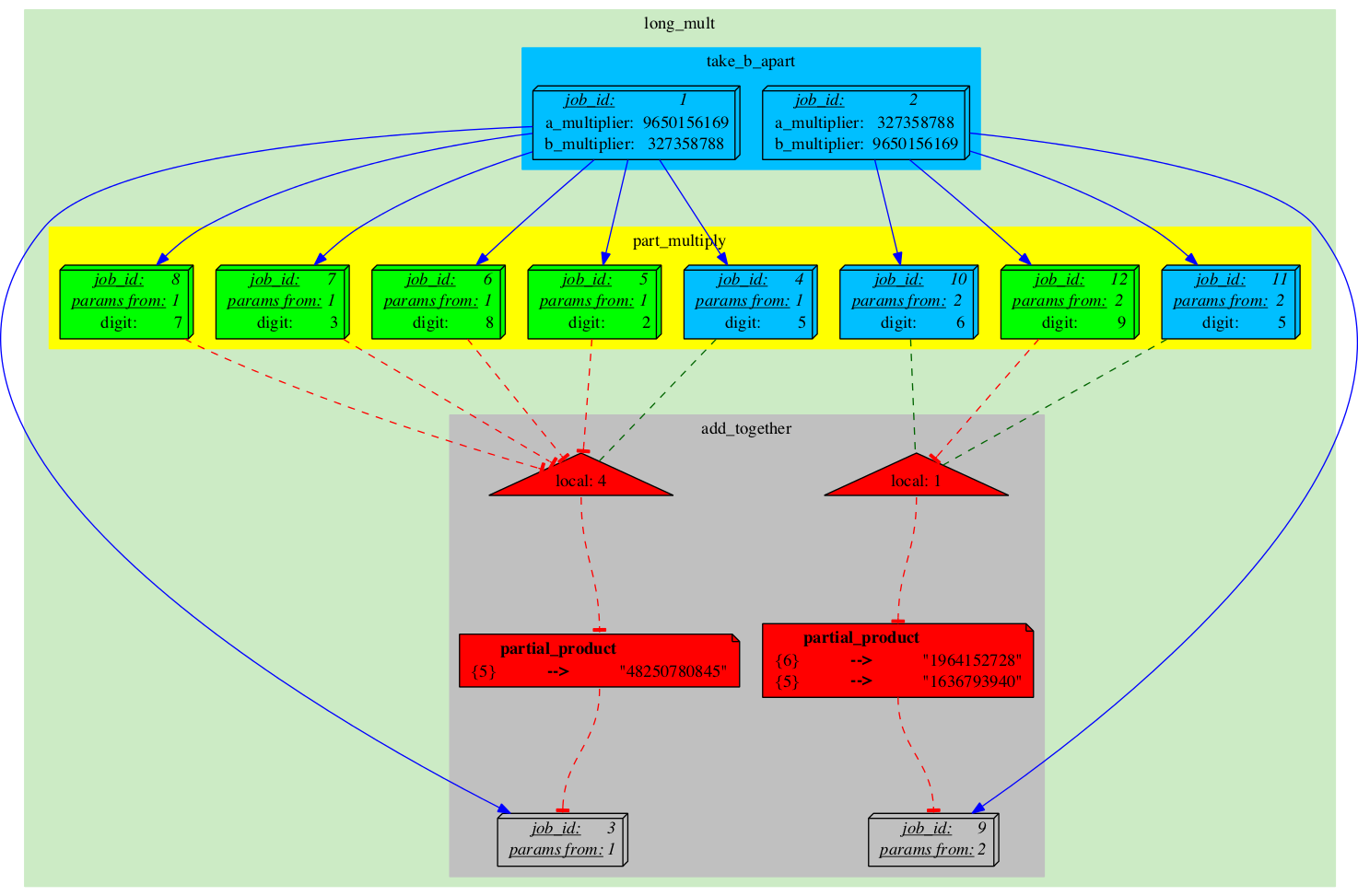
A couple more Jobs get executed with a similar effect
|

|
|
After executing these two jobs:
|
And another couple more Jobs...
|
|
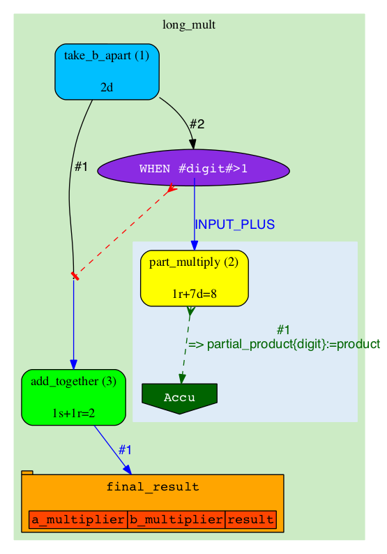
Finally, one of the Semaphores gets completely unblocked, which turns Job_9 into 'READY' state.
|
|
|
To recap:
|
|
Job_9 gets executed.
|
|
|
We can see that the stream of execution starting at Job_2 finished first. In general, there is no guarantee for the order of execution of jobs that are in 'READY' state. |
|
The last 'part_multiply' job gets run...
|
|
|
Job_3 gets executed.
|
|
|
The result also goes into 'final_result' table. We can verify that the two results are identical. |