- Analysis happens in walled gardens (Gromacs, Amber, VMD)
- Exclusively command line interfaces, C and Fortran code
- Duplication of statistical algorithms by non-experts (e.g. chemists, biologists)
- Possible code maintainability issues?
Carlos X. Hernández, Matthew P. Harrigan, M. Muneeb Sultan, Brooke E. Husic
Updated: Jun. 23, 2016 (msmbuilder v3.5)
Old-School Analysis of MD Data
Jarvis Patrick Clustering in Gromacs
real code in gromacs
static void jarvis_patrick(int n1, real **mat, int M, int P,
real rmsdcut, t_clusters *clust) {
t_dist *row;
t_clustid *c;
int **nnb;
int i, j, k, cid, diff, max;
gmx_bool bChange;
real **mcpy = NULL;
if (rmsdcut < 0) {
rmsdcut = 10000;
}
/* First we sort the entries in the RMSD matrix row by row.
* This gives us the nearest neighbor list.
*/
Jarvis Patrick Clustering in Gromacs (Cont.)
// Five more pages of this
// You get the idea

// Also, how do we even use this function?
static void jarvis_patrick(int n1, real **mat, int M, int P,
real rmsdcut, t_clusters *clust);
Enter Data Science
- Machine learning is mainstream now!
- Thousands of experts are using machine learning approaches
- Well-tested, performant, and facile implementations are available
- Writing your own is not the way to go!
- E.g: Is clustering that special and MD-specific such that we need our own custom algorithms and implementations?
MSMBuilder3: Design
Builds on scikit-learn idioms:
- Everything is a
Model. - Models are
fit()on data. - Models learn
attributes_. Pipeline()concatenate models.- Use best-practices (cross-validation)
Everything is a Model()!
>>> import msmbuilder.cluster
>>> clusterer = msmbuilder.cluster.KMeans(n_clusters=4)

>>> import msmbuilder.decomposition
>>> tica = msmbuilder.decomposition.tICA(n_components=3)

>>> import msmbuilder.msm
>>> msm = msmbuilder.msm.MarkovStateModel()
Hyperparameters go in the constructor.
Models fit() data!
>>> import msmbuilder.cluster

>>> trajectories = [np.random.normal(size=(100, 3))]

>>> clusterer = msmbuilder.cluster.KMeans(n_clusters=4, n_init=10)
>>> clusterer.fit(trajectories)

>>> clusterer.cluster_centers_

array([[-0.22340896,  1.0745301 , -0.40222902],
       [-0.25410827, -0.11611431,  0.95394687],
       [ 1.34302485,  0.14004818,  0.01130485],
       [-0.59773874, -0.82508303, -0.95703567]])
Estimated parameters always have trailing underscores!
fit() acts on lists of sequences
>>> import msmbuilder.msm

>>> trajectories = [np.array([0, 0, 0, 1, 1, 1, 0, 0])]

>>> msm = msmbuilder.msm.MarkovStateModel()
>>> msm.fit(trajectories)

>>> msm.transmat_

array([[ 0.75      ,  0.25      ],
       [ 0.33333333,  0.66666667]])
This is different from sklearn, which uses 2D arrays.
Models transform() data!
>>> import msmbuilder.cluster

>>> trajectories = [np.random.normal(size=(100, 3))]

>>> clusterer = msmbuilder.cluster.KMeans(n_clusters=8, n_init=10)
>>> clusterer.fit(trajectories)
>>> Y = clusterer.transform(trajectories)

[array([5, 6, 6, 0, 5, 5, 1, 6, 1, 7, 5, 7, 4, 2, 2, 2, 5, 3, 0, 0, 1, 3, 0,
        5, 5, 0, 4, 0, 0, 3, 4, 7, 3, 5, 5, 5, 6, 1, 1, 0, 0, 7, 4, 4, 2, 6,
        1, 4, 2, 0, 2, 4, 4, 5, 2, 6, 3, 2, 0, 6, 3, 0, 7, 7, 7, 0, 0, 0, 3,
        3, 2, 7, 6, 7, 2, 5, 1, 0, 3, 6, 3, 2, 0, 5, 0, 3, 4, 2, 5, 4, 1, 5,
        5, 4, 3, 3, 7, 2, 1, 4], dtype=int32)]
Moving the data-items from one "space" / representation into another.
Pipeline() concatenates models!
>>> import msmbuilder.cluster, msmbuilder.msm
>>> from sklearn.pipeline import Pipeline

>>> trajectories = [np.random.normal(size=(100, 3))]

>>> clusterer = msmbuilder.cluster.KMeans(n_clusters=2, n_init=10)
>>> msm = msmbuilder.msm.MarkovStateModel()
>>> pipeline = Pipeline([("clusterer", clusterer), ("msm", msm)])

>>> pipeline.fit(trajectories)
>>> msm.transmat_

array([[ 0.53703704,  0.46296296],
       [ 0.53333333,  0.46666667]])
Data "flows" through transformations in the pipeline.
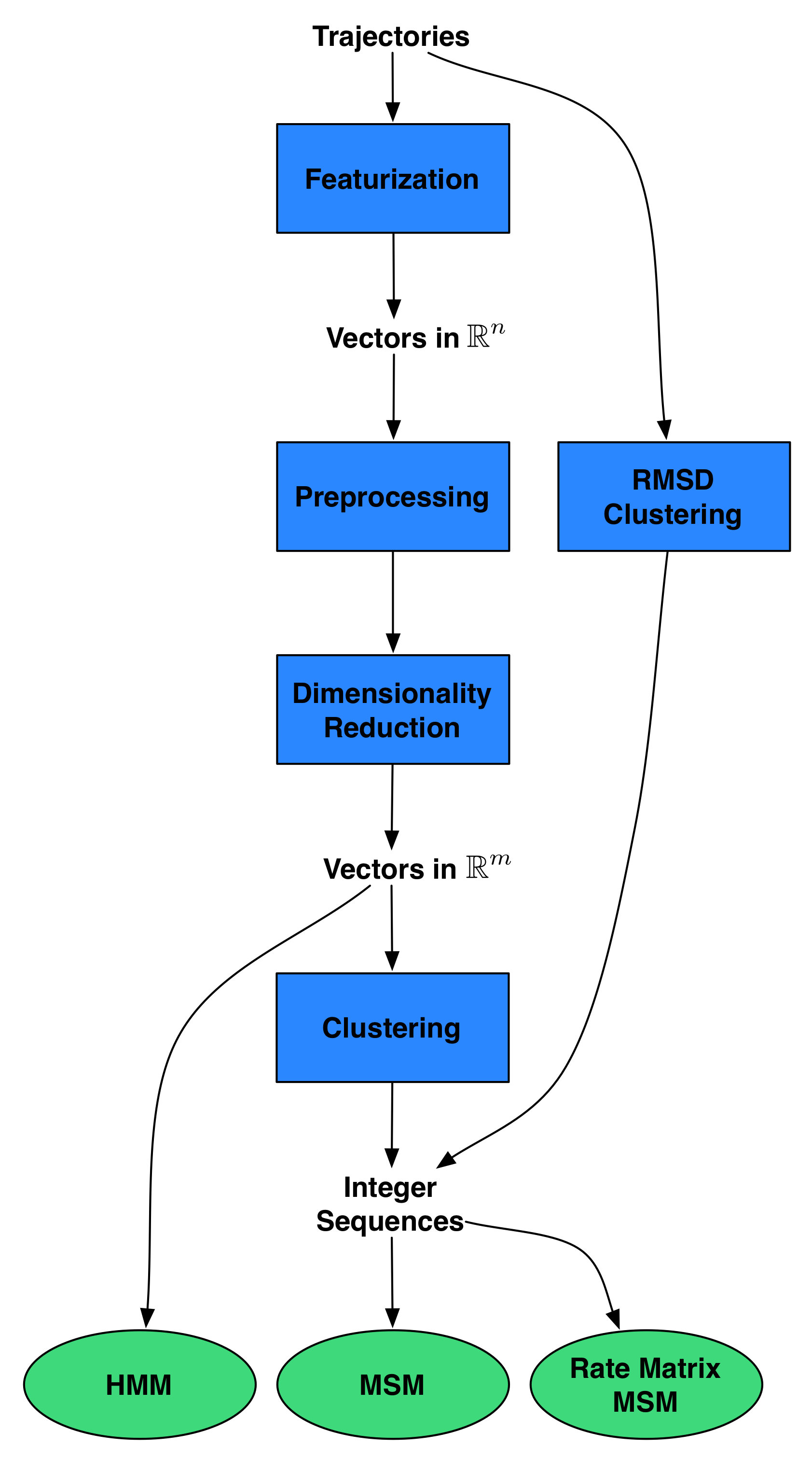
Loading Trajectories
You can use MDTraj to load your trajectory files
>>> import glob
>>> import mdtraj as md

>>> filenames = glob.glob("./Trajectories/ala_*.h5")
>>> trajectories = [md.load(filename) for filename in filenames]
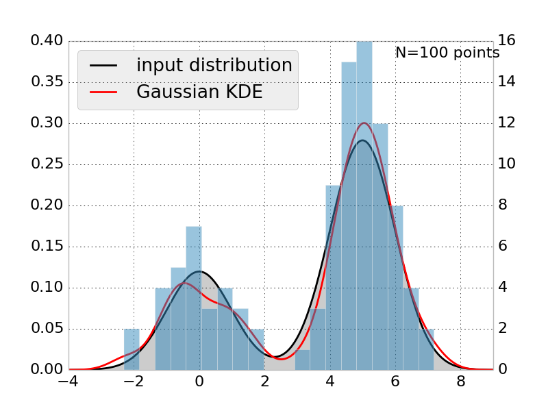
Featurization
Featurizers wrap MDTraj functions via the transform() function
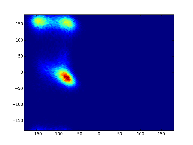
>>> from msmbuilder.featurizer import DihedralFeaturizer
>>> from matplotlib.pyplot import hexbin, plot

>>> featurizer = DihedralFeaturizer(
...        ["phi", "psi"], sincos=False)
>>> X = featurizer.transform(trajectories)
>>> phi, psi = np.rad2deg(np.concatenate(X).T)

>>> hexbin(phi, psi)
Featurization (Cont.)
You can even combine featurizers with FeatureSelector
>>> from msmbuilder.featurizer import DihedralFeaturizer, ContactFeaturizer
>>> from msmbuilder.feature_selection import FeatureSelector

>>> dihedrals = DihedralFeaturizer(
...         ["phi", "psi"], sincos=True)
>>> contacts = ContactFeaturizer(scheme='ca')
>>> featurizer = FeatureSelector([('dihedrals', dihedrals),
...                               ('contacts', contacts)])
>>> X = featurizer.transform(trajectories)
Preprocessing
Preprocessors normalize/whiten your data
>>> from msmbuilder.preprocessing import RobustScaler
>>> scaler = RobustScaler()

>>> Y = scaler.transform(X)
This is essential when combining different featurizers!
Also check out MinMaxScaler and StandardScaler
Decomposition
Reduce the dimensionality of your data
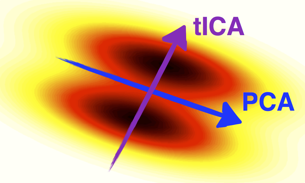
of freedom in time-series data
>>> from msmbuilder.decomposition import tICA

>>> tica = tICA(n_components=2, lagtime=5)
>>> Y = tica.fit_transform(X)
Also check out PCA and SparseTICA
Markov State Models
We offer two main flavors of MSM:
MarkovStateModel- Fits a first-order Markov model to a discrete-time integer labeled timeseries.ContinuousTimeMSM- Estimates a continuous rate matrix from discrete-time integer labeled timeseries.
Each has a Bayesian version, which estimates the error associated with the model.
Hidden Markov Models
We also offer two types of HMMs:
GaussianHMM- Reversible Gaussian Hidden Markov Model L1-Fusion RegularizationVonMisesHMM- Hidden Markov Model with von Mises Emissions
HMMs are great for macrostate modeling!
Cross-Validation
from sklearn.cross_validation import ShuffleSplit

cv = ShuffleSplit(len(trajectories), n_iter=5, test_size=0.5)

for fold, (train_index, test_index) in enumerate(cv):
    train_data = [trajectories[i] for i in train_index]
    test_data = [trajectories[i] for i in test_index]
    model.fit(train_data)
    model.score(test_data)
Also check out scikit-learn's KFold, GridSearchCV and RandomizedSearchCV.
Command-line Tools
We also offer an easy-to-use CLI for the API-averse
$ msmb DihedralFeaturizer --top my_protein.pdb --trjs "*.xtc" \
    --transformed diheds --out featurizer.pkl

$ msmb tICA -i diheds/ --out tica_model.pkl \
    --transformed tica_trajs.h5 --n_components 4

$ msmb MiniBatchKMeans -i tica_trajs.h5 \
    --transformed labeled_trajs.h5 --n_clusters 100

$ msmb MarkovStateModel -i labeled_trajs.h5 \
   --out msm.pkl --lag_time 1
Related Projects
We also maintain:
Osprey
Fully-automated, large-scale hyperparameter optimization

Osprey: Estimator
Define your model
estimator:
  # The model/estimator to be fit.

  eval_scope: msmbuilder
  eval: |
    Pipeline([
            ('featurizer', DihedralFeaturizer(types=['phi', 'psi'])),
            ('scaler', RobustScaler()),
            ('tica', tICA(n_components=2)),
            ('cluster', MiniBatchKMeans()),
            ('msm', MarkovStateModel(n_timescales=5, verbose=False)),
    ])
Osprey: Search Strategy
Choose how to search over your hyperparameter space
strategy:

    name: gp  # or random, grid, hyperopt_tpe
    params:
      seeds: 50
Osprey: Search Space
Select which hyperparameters to optimize
search_space:
  featurizer__types:
    choices:
      - ['phi', 'psi']
      - ['phi', 'psi', 'chi1']
    type: enum

  cluster__n_clusters:
    min: 2
    max: 1000
    type: int
    warp: log # search over log-space
Osprey: Cross-Validation
Pick your favorite cross-validator
cv:
  name: shufflesplit # Or kfold, loo, stratifiedshufflesplit, stratifiedkfold, fixed
  params:
    n_iter: 5
    test_size: 0.5
Osprey: Dataset Loader
Load your data, no matter what file type
dataset_loader:
  # specification of the dataset on which to train the models.
  name: mdtraj # Or msmbuilder, numpy, filename, joblib, sklearn_dataset, hdf5
  params:
    trajectories: ./fs_peptide/trajectory-*.xtc
    topology: ./fs_peptide/fs-peptide.pdb
    stride: 100
Osprey: Trials
Save to a single SQL-like database, run on as many clusters as you'd like*
trials:
  # path to a database in which the results of each hyperparameter fit
  # are stored any SQL database is supported, but we recommend using
  # SQLLite, which is simple and stores the results in a file on disk.
  uri: sqlite:///osprey-trials.db
Osprey: Running a Job
Simple command-line interface, easy to run on any cluster
$ osprey worker -n 100 config.yaml
...
----------------------------------------------------------------------
Beginning iteration                                           10 / 100
----------------------------------------------------------------------
Loading trials database: sqlite:///trials.db...
History contains: 9 trials
Choosing next hyperparameters with gp...
  {'tica__n_components': 2, 'tica__lag_time': 180, 'cluster__n_clusters': 36}
(gp took 0.000 s)
...
Success! Model score = 4.214510
(best score so far   = 4.593165)
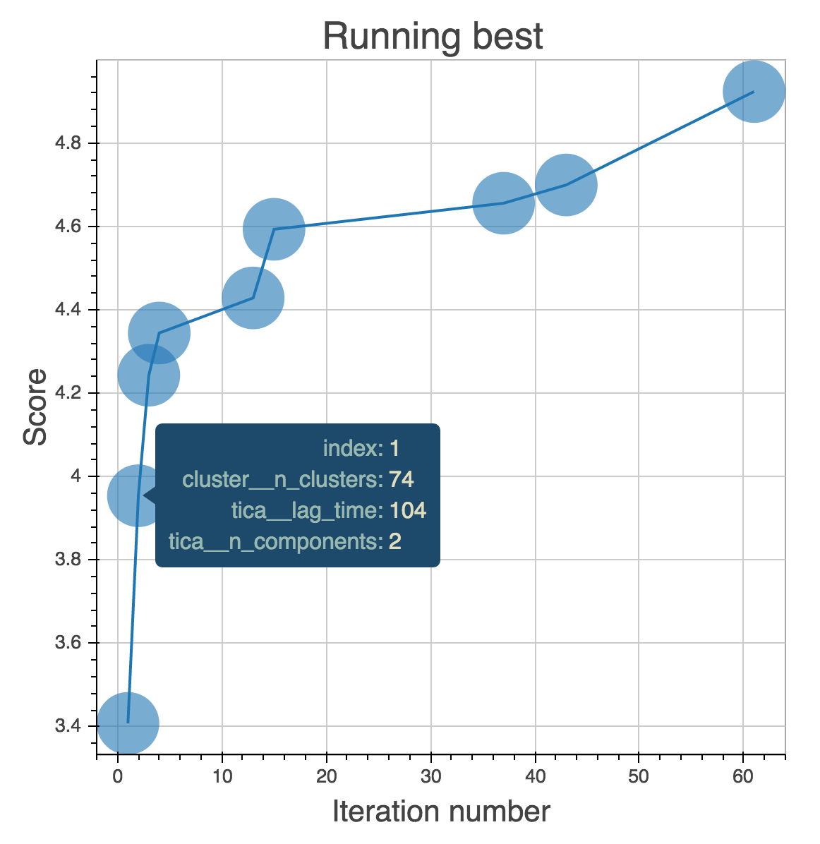
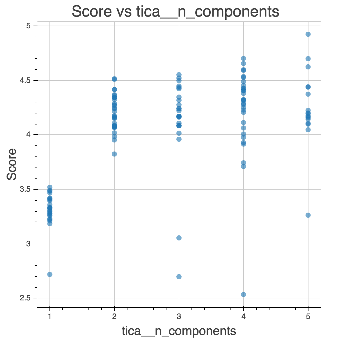
Osprey: Real-Time Analytics
Osprey also makes it easy to create interactive dashboards
$ osprey plot config.yaml